Analysis of a Delayed Stochastic One Predator Two Prey Population Model in a Polluted Environment

(1)

https://www.scirp.org/journal/jamp

ISSN Online: 2327-4379 ISSN Print: 2327-4352

DOI: 10.4236/jamp.2019.710154 Oct. 14, 2019 2265 Journal of Applied Mathematics and Physics

Analysis of a Delayed Stochastic One-Predator

Two-Prey Population Model in a Polluted

Environment

Mengwei Li, Yuanfu Shao, Yafei Yang

College of Physics, Guilin University of Technology, Guilin, China

Abstract

This paper is concerned with the dynamics of a delayed stochastic one-predator two-prey population model in a polluted environment. We show that there exists a unique positive solution that is permanent in time average under certain conditions. Moreover, the global attractively of system is studied. Finally, some numerical simulations are given to illustrate the main results.

Keywords

Random Perturbations, Time Delays, Pollution, Permanent in Time Average

1. Introduction

With the rapid development of economy, environmental pollution has gradually become the major social problem today. With a growing number of toxicant and contaminants entering into the ecosystem, the quality of our living environment has declined. Then many species have been extinct, and some of them are on the edge of extinction. Therefore, controlling environment pollution has become a major topic in many countries, which draws researchers to investigate the influ-ence of environment pollution.

In the 1980s, Hallam et al. [1] [2] [3] firstly proposed the deterministic models to study the impact of environment toxicant on the survival of biological popu-lation. Their studies have provided useful bases about protecting species for us. However, population system is often affected by environmental noise, and there are many scholars who have studied the dynamics of stochastic models with toxicant [4] [5] [6] [7].

On the other hand, more realistic models of population interactions should

How to cite this paper: Li, M.W., Shao, Y.F. and Yang, Y.F. (2019) Analysis of a Delayed Stochastic One-Predator Two-Prey Population Model in a Polluted Environ-ment. Journal of Applied Mathematics and Physics, 7, 2265-2282.

https://doi.org/10.4236/jamp.2019.710154

Received: August 31, 2019 Accepted: October 11, 2019 Published: October 14, 2019

http://creativecommons.org/licenses/by/4.0/

(2)

DOI: 10.4236/jamp.2019.710154 2266 Journal of Applied Mathematics and Physics take the effects of time delay into account [8] [9]. Further, in the natural world, it is a common phenomenon that a predator feeds on some competing preys [10] [11] [12]. However, there is little research on the delayed stochastic one-predator two-prey model in a polluted environment. Thus we consider a stochastic de-layed one-predator two-prey model with toxicant input in this article.

The rest is organized as follows. In Section 2, we show some notations and in-troduce a stochastic delayed one-predator two-prey model in polluted environ-ment. In Section 3, we show that the system (SM) has a unique global positive solution. In Section 4, we give the main theorems and their proof. In Section 5, the attractively global system is investigated. In Section 6, we present numerical simulations to illustrate our mathematical findings.

2. The Model and Notations

In this section, we will give some notations on stochastic one-predator-two-prey system. The stochastic predator-prey system in a polluted environment takes the following form:

( )

( ) (

) ( )

( )

( ) (

) ( )

( )

( ) ( )

1 1 1 1 1 11 1 12 2

2 2 2 2 2 21 1 22 2

1 1 1 1 1

2 1 2 2 2

d d ,

d d .

e

e e

x t x t r a C t c x t c x t t x t x t r a C t c x t c x t t

C t k C t g m C t t

C t k C t g m C t t

C t hC t u t t

 = _ − − − _



 = _− − + − _

 ₌_ ₋ ₊ _

 _ _



= − + 

  

 _{= −}_ ₊ _

  



(2.1)

The above model does not incorporate the effect of time delay, but for a long time, it has been recognized that delays can have a complex effect on the dy-namics of a system [9] [13]. In the same time, the natural growth of many popu-lations is inevitably affected by many random disturbances. Considering the ef-fects of random disturbances, we assume the growth rate of prey and the death rate of predator are perturbed with

( )

, 1, 2, 3.

i i i i

r → +r βB t i=

where B ti

( )(

i=1, 2, 3

)

is mutually independent one-dimensional standard

Brownian motions with Bi

( )

0 =0 and β >i 0

(

i=1, 2, 3

)

being the intensities

of white noises. Stochastic version corresponding to deterministic system with time delays can be rewritten as:

( )

(

)

( )

(

)

( )

( ) (

) ( )

( )

( ) (

) ( )

( )

( ) ( )

1 1 1 1 1 11 1 12 2 1 1 1

2 2 2 2 2 21 1 22 2 2 2 2

1 1 1 1 1

2 1 2 2 2

d d d ,

d d ,

d d .

e

e e

x t x t r a C t c x t c x t t x t B t

x t x t r a C t c x t c x t t x t B t

C t k C t g m C t t

C t k C t g m C t t

τ β

 = _ − − − − _ +



 = _− − + − − _ +

 ₌_ ₋ ₊ _

  



= − + 

  



= − + 

  



(2.2)

(3)

preda-DOI: 10.4236/jamp.2019.710154 2267 Journal of Applied Mathematics and Physics tor-prey system with time delays and toxicant inputs in the same time. Therefore, on the basis of article [14], we establish the following delayed stochastic one-predator two-prey model in a polluted environment:

( )

(

)

(

)

( )

(

)

( )

(

)

( )

(

)

(

)

( )

1 1 1 1 0 11 1 12 2 12 13 3 13 1 1 1

2 2 2 2 0 21 1 21 22 2 23 3 23 2 2 2

3 3 3 3 0 31 1 31 32 2 32 33 3 3 3 3

0 1 1

d d d ,

d _e

x t x t r a C t c x t c x t c x t t x t B t

x t x t r a C t c x t c x t c x t t x t B t

x t x t r a C t c x t c x t c x t t x t B t

C t k C t

τ τ β

ρ

 

= _ − − − − − − _ +

 

= _ − − − − − − _ +

 

= _− − + − + − − _ +

= +

(

) ( )

( )

( ) ( )

1 1 1 0 d ,

d _e _e d .

k g m C t t

θβ 

    

− +

 

  

 _{= −}_ ₊ _

  



(2.3) with initial data

( )

,

[

, 0 ,

]

max

{ }

, , 1, 2, 3.

i i ij

x θ =ξ θ θ∈ −τ τ= τ i j=

where x ti

( )

is the size of the the prey i, i=1, 2, and x t3

( )

is the size of the

predator; ri is the growth rate of the i the species, i=1, 2, r3 is the death rate

of the predator; cii is the intra-specific competition rate, i=1, 2, 3. c12 and 21

c stand for the inter-specific competition rates between species 1 and 2, c13

and c23 stand for the capture rates, c31 and c32 are the efficiency of food

conversion. C t0

( )

and C te

( )

denote the concentrations of the toxicant in the

organism of species and the environment at time t, respectively. ai stand for

dose-response of the prey and predator to the organismal toxicant, and −gi

and −mi denote the excretion and depuration rates of the toxicant, i=1, 2, 3,

respectively. k1 and ρ1 represent the absorption of toxicant per unit of mass

by the environment and by food, respectively. θ is the concentration of tox-icant in the environment; β is the uptake rate of food per unit mass. Parameter h reflects the ability of the environment to clean up toxicant. u t

( )

denotes the

exogenous rate of toxicant input into the environment and it is supposed to be bounded and 0≤U1≤u t

( )

≤U2 < ∞. All coefficients mentioned above are

posi-tive constants. τ_ij >0 represents the time delay.

( )

(

1

( ) ( ) ( )

, 2 , 3

)

ξ θ = ξ θ ξ θ ξ θ Τ∈U, where U represents the space of all the continued functions from

[

−τ, 0

]

to R3+=

{

x=

(

x x x1, 2, 3

)

∈R x3 i >0,i=1, 2, 3

}

.

Although the model is a five-dimensional system, because the explicit solu-tions of the latter two equasolu-tions are easy to get, it is actually only necessary to study the first three stochastic differential equations of the model, which is called model (SM) in this paper.

For the sake of simplification, we define some notations:

2 2

3

3 3

, 1, 2, ,

2 2

i i i

b = −r β i= b = +r β

0, 1, 2, 3, 22 31 1 11 32 2 11 22 3,

i i i

d = −b a C i= ∆ =c c b +c c b −c c b

2

11 1 1 11 12 13

2

21 2 2 21 22 23

2

31 3 3 31 32 33

2

2 , ,

2

c r c c c

c r C c c c

c r c c c

β β β

= =

− − − −

(4)

DOI: 10.4236/jamp.2019.710154 2268 Journal of Applied Mathematics and Physics

1 12 13 11 1 13 11 12 1

1 2 22 23 2 21 2 23 3 21 22 2

3 32 33 31 3 33 31 32 3

, , ,

r c c c r c c c r

C r c c C c r c C c c r

r c c c r c c c r

= = =

− − − − − − −

2 2 2

1 12 13 11 1 13 11 12 1

2 2 2

1 2 22 23 2 21 2 23 3 21 22 2

2 2 2

3 32 33 31 3 33 31 32 3

2 2 2

2 , 2 , 2 .

2 2 2

c c c c c c

C c c C c c C c c

c c c c c c

β β β

= = =

− − − −

  

For a function g, we denote the following notations:

( )

*

( )

0 0 0

1 1 1

d , lim sup d , lim inf d .

t t t

t t

g t g s s g t g s s g t g s s

t _→∞ t ∗ →∞ t

=

_∫

=

_∫

=

_∫

3. Existence and Uniqueness of the Global Positive Solution

In order to make the model be sense, we need to show the solution is non-negative and global.

Lemma 3.1 ([15]) For model (2.3), if 0< +k1 ρ θβ1 k1<g1+m1, U2≤h,

then 0≤C0

( )

t ≤1, 0≤C te

( )

≤1.

This paper assumes that condition 0< +k1 ρ θβ1 k1<g1+m1, U2 ≤h is

al-ways true in model (2.3), then the solution process of model (SM) should be non-negative.

Lemma 3.2 For any initial value

( )

(

( ) ( ) ( )

)

3

1 , 2 , 3 R

ξ θ = ξ θ ξ θ ξ θ Τ∈ ₊, there is a unique global positive solution

(

( ) ( ) ( )

)

3

1 , 2 , 3 , . .

x t x t x t ∈R a s+ . Moreover, there

is a positive constants k such that

( )

(

)

lim sup E i , 1, 2, 3.

t

x t k i

→∞ ≤ = (3.1)

Proof. Consider the following system:

( )

( ) ( ) ( )

_{( )}

( )

( ) ( ) ( )

_{( )}

( )

( ) ( ) ( )

_{( )}

3 13

1 2 12

1 23

1 21 2

1 31 2 32 3

1 1 1 0 11 12 13 1 1

2 2 2 0 21 22 23 2 2

3 3 3 0 31 32 33 3 3

d e e e d d ,

d e e e d d .

N t

N t N t

N t

N t N t

N t N t N t

N t r a C t c c c t B t

N t r a C t c c c t B t

τ τ

β

β −

−

− −

 =_ − − − − _ +



 ₌_ ₋ ₋ ₋ ₋ _ ₊

 _ _



 

 = − −_ + + − _ +



(3.2)

with initial value N_i

( )

θ =logξ θ_i

( )

,i=1, 2, 3. Since the coefficients of (3.2) obey

the local Lipstchiz condition, then (3.2) has a unique local positive solution

( )

N t on

[

0,τ_e

)

, where τe stands for the explosion time. Hence it follows

from Itô’s formula that (SM) has the following unique positive global solution

( )

(

( )

1( )

_{( )}

2( )

_{( )}

3( )

)

Τ

1 e , 2 e , 3 e .

N t N t N t

x t = x t = x t = x t =

Now we show that x t

( )

is global, i.e., τe= ∞. Consider the following

sys-tem:

( )

(

)

(

)

( )

1 1 1 1 0 11 1 1 1 1

2 2 2 2 0 22 2 2 2 2

3 3 3 3 0 31 1 31 32 3 32 33 3 3 3 3

d d d ,

d d d .

y t y t r a C t c y t t y t B t

y t y t r a C t c y t t y t B t

y t y t r a C t c y t c y t c y t t y t B t

β β

τ τ β

 = _ − − _ +

 ₌ _ ₋ ₋ _ ₊

 _ _



 

= − − + − + − − +

  



(5)

DOI: 10.4236/jamp.2019.710154 2269 Journal of Applied Mathematics and Physics with initial value y_i

( )

θ =ξ θ_i

( )

,i=1, 2, 3. By the stochastic comparison

theo-rem [16], one can see that for t∈

[

0,τ_e

)

,

( )

, . ., 1, 2, 3.

i i

x t ≤y t a s i=

Thanks to Theorem 4.2 in [17], system (3.3) can be explicitly solved as follows

( )

{

( )

}

( )

{

( )

}

( )

{

( )

}

( )

{

( )

}

( )

{

(

)

(

)

( )

}

( )

{

(

)

(

)

( )

}

1 1 1 1

1

1 11 ₀ 1 1 1

2 2 2

2

1

2 22 ₀ 2 2 2

3 ₀ 31 1 31 32 2 32 3 3

3

1

2 33 ₀ 3 ₀ 31 1 31 32 2 32 3 3

exp

,

0 exp d

exp

,

0 exp d

exp d

.

0 exp d d

t

t s

d t B t y t

y c d s B s s

d t B t y t

y c d s B s s

d t c y s c y s s B t

y t

y c d s c y u c y u u B s s

β β β

β

τ τ β

−

 +

= 

 + +



 +

= 

 ₊ ₊



 ₋ ₊ ₋ ₊ ₋ ₊

 = 

 + − + − + − +



∫

Note that y t1

( ) ( )

,y2 t and y t3

( )

are existent on t≥0, hence τe= +∞.

Before we state the main theorem of this paper, we need to introduce several hypotheses.

Hypothesis 1. C>0,Ci >0,i=1, 2, 3. which imply that all the populations

coexist if model (_{SM) frees from stochastic noises.}

Hypothesis 2. c11>c12+c13,c22>c21+c23,c33>c31+c32.

4. Permanence in Time Average

In this section, we study the permanent in time average of systems (2.3) and (SM). We firstly do some preparation.

Definition 4.1. System (2.3) is said to be permanent in time average if there are positive constants si and vi (i=1, 2, 3) such that

( )

lim inf lim sup , 1, 2, 3.

i i i i

t _t

v x t x t s i

→∞ _→∞

≤ ≤ ≤ =

holds for any solution

(

x t1

( ) ( ) ( )

,x t2 ,x t3

)

of system (2.3) with initial

condi-tion

( )

{

(

( ) ( ) ( )

)

}

(

[

]

2

)

1 , 2 , 3 : 0 , 0 : .

t t t t t C R

ξ = ξ ξ ξ − ≤ ≤τ ∈ −τ +

Lemma 4.1 ([18]). Suppose x t

( )

be a continuous function from Ω 0,×

[

+∞

)

to R₊.

1) If there exist constants λ λ, 0 >0 and T>0 such that

( )

_{0 0}

( )

1

log d ,

n t

i i i

x t λ λt x s s βB t

=

≤ −

_∫

+

∑

for t≥T, where B t_i

( )

are independent standard Brownian motions and β_i

are constants, 1≤ ≤i n, then we have:

( )

*

0, . ., if 0,

lim 0, . ., if 0.

t

x a s

x t a s

λ λ λ

λ →∞

 ≤ ≥



 ₌ _<



2) If there exist positive constants λ λ, 0 and T such that

( )

_{0 0}

( )

1

log d ,

n t

i i i

x t λ λt x s s βB t

=

(6)

DOI: 10.4236/jamp.2019.710154 2270 Journal of Applied Mathematics and Physics for all t≥T, where B t_i

( )

are independent standard Brownian motions and

i

β are constants, 1≤ ≤i n, then if λ≥0, we have x*≥λ λ0, . .a s .

Lemma 4.2 For arbitrary τ ≥0, we have

( )

1

lim _tt i d 0, . ., 1, 2.

t→∞_t

∫

−τy s s= a s i= (4.1)

Proof. Consider the first two equations in model (3.3). By [19], we have

( )

2

0

2

1

lim d . ., if , 1, 2,

2

lim 0 . ., if , 1, 2.

2

t

i i

t

ii

i

i i

t

a

y s s a s b i

t c

y t a s b i

β

β →∞

→∞ 

= ≥ =

  

 ₌ _< ₌



∫

Consequently, if 2

2

i i

b <β , then

( )

(

₀

( )

₀

( )

)

1 1

lim _tt i d lim t i d t i d 0.

t _t y s s t _t y s s y s s

τ τ

− −

→+∞

∫

= →+∞

∫

−

∫

=

If 2

2

i i

b ≥β , then

( )

(

₀

( )

₀

( )

)

1 1

lim t d lim t d t d i i 0.

i i i

t

t t

ii ii

a a

y s s y s s y s s

t t c c

τ τ

− −

→+∞

∫

= →+∞

∫

−

∫

= − =

We now consider the following stochastic equation with delays

( )

(

( )

)

( )

(

( )

)

( )

(

)

(

)

( )

)

( )

(

[

]

)

( )

(

[

]

)

( )

(

[

]

)

1 1 1 11 1 1 1

2 2 2 22 2 2 2

3 3 3 31 1 31 32 2 32 33 3 3 3

1 1

2 2

3 3

d d d ,

, 0 ; ,

, 0 ; .

y t y t r c y t t B t

y t y t r c y t t B t

y t y t r c y t c y t c y t t B t

y t t C R

y t t C R

y t t C R

β β

τ τ β

ξ τ

+

 = _ − + _



 = _ − + _



 ₌ _ _{− +} ₋ ₊ ₋ ₋ ₊ _

 _ _



 = ∈ −



= ∈ −

 

= ∈ −



(4.2) Lemma 4.3 Assume that b1≥0,b2≥0 and

31 1 11 32 2 22 3 0

c b c +c b c − ≥b , then the solution of (4.2) has the following

proper-ties:

( )

1

( )

2

( )

1 2 3

11 22 11 22 33

lim , lim , lim ,

t t t

b b

y t y t y t

c c c c c

→∞ →∞ →∞

∆

= = =

( )

₍

₎

log

lim i 0, . . 1, 2, 3 .

t

y t

a s i

t

→∞ = =

Proof. The solution of (4.2) has the property that ([4])

( )

_{( )}

1 1

1 11

log

lim 0, lim ,

t t

y t b

y t

t c

→∞ = →∞ = (4.3)

By Itô’s formula, we get

( )

1 1 1 11 ₀ 1 1 1

(7)

( )

2 2 2 22 ₀ 2 2 2

logy t −logy 0 =b t−c

∫

ty s ds+β B t , (4.5)

( )

(

)

(

)

( )

31

31 32 32

3 3

3 31 ₀ 1 31 32 ₀ 2 32 33 ₀ 3 2 2

3 31 ₀ 1 32 ₀ 2 33 ₀ 3 31 1

0

1 32 2 2 3 3

log log 0

d d d

d d d d

d d d .

t t t

t t t t

t

t t

t

y t y

b t c y s s c y s s c y s s B t

b t c y s s c y s s c y s s c y s s

y s s c y s s y s s B t

τ

τ τ τ

τ τ β

β

−

− − −

−

= − + − + − − +



= − + + − − _

  

− _− _ − _+

  

∫

(4.6)

Dividing both sides of (4.4), (4.5) and (4.6) by t, one can see that

( )

1 1 1

1 11 1 1

1

log ,

0

y t B t

b c y t

t y t

β

= − + _(4.7)

( )

2 2 2

2 22 2 2

1

log ,

0

y t B t

b c y t

t y t

β

= − + (4.8)

( )

31 31

32 32

3 3

0 31

3 31 1 32 2 33 3 1 1

0 ₃ ₃

32

2 2

1 log

0

d d

d d .

t t

y t

t y

c

b c y t c y t c y t y s s y s s

t B t c

y s s y s s

t t

τ τ

β

− −

 

= − + + − − _ − _

 

 

− _ − _+

 

∫

(4.9)

And it is well known that

( )

lim i 0, . ., 1, 2, 3.

t

B t

a s i

t

→∞ = = (4.10)

Utilizing Lemma 4.1, 2

1 1 1 2 0

b = −r β ≥ and b2= −r2 β22 2≥0, it is easy to

derive that

( )

1

1 0

11

1

lim t d , . ..

t

b

y s s a s

t c

→∞

∫

= (4.11)

And

( )

2

2 0

22

1

lim t d , . ..

t

b

y s s a s

t c

→∞

∫

= (4.12)

Plugging (4.11), (4.12) into (4.7), (4.8), respectively, then combining (4.10) leads to

( )

1

log

lim 0, . ..

t

y t

a s t

→∞ = (4.13)

and

( )

2

log

lim 0, . ..

t

y t

a s t

→∞ = (4.14)

Besides, computing

( )

4.7 ×c c22 31+

( )

4.8 ×c c11 32+

( )

4.9 ×c c11 22, one can derive

(8)

( )

31 31

32 32

1 2 3

22 31 11 32 11 22

1 2 3

0 11 22 31

1 1

0 11 22 32

2 2

1 1 2 2

22 31 1 11 1 11 32 2 22 2

11 22 3

log log log

0 0 0

d d

t t t t

y t y t y t

c c c c c c

t y t y t y

c c c

y s s y s s

t c c c

y s s y s s

t

B t B t

c c b c y t c c b c y t

t t

c c b

τ τ

β β

− −

+ +

 

+ _ − _

 

 

+ _ − _

 

   

= _ − + _+ _ − + _

   

+ −

∫

( )

3 3

( )

31 1 32 2 33 3

B t

c y t c y t c y t

t β

 

+ + − +

 

 

( )

22 31 1 11 32 2 11 22 3 11 22 31 1 11 22 32 2

1 1 11 22 31 1 11 22 32 2 11 22 33 3 22 31

2 2 3 3

11 31 11 22

1 1 2 2 3 3

11 22 33 3 22 31 11 31 11 22 .

c c b c c b c c b c c c y t c c c y t B t c c c y t c c c y t c c c y t c c

t

B t B t

c c c c

t t

B t B t B t

c c c y t c c c c c c

t t t

β

β β

β β β

= + − − −

+ + − +

+ +

= ∆ − + + +

(4.15)

In view of (4.1), (4.13), (4.14), (4.15) and Lemma 4.1, we can gain that

( )

3 31 1 11 32 2 22 3

0

11 22 33

lim 0, . ., if 0,

1

lim d , . ., if 0.

t t t

y t a s c b c c b c b

y s s a s c b c c b c b

t c c c

→∞

 = + − <



 ₌ ∆ ₊ _{− ≥}





∫

(4.16)

By (3.11)-(3.16), we have

( )

3

log

lim 0, . ..

t

y t

a s t

→∞ =

This completes the proof.

Lemma 4.4 For arbitrarily τ≥0,

( )

3

1

lim t d 0, . ..

t

t→∞_t

∫

−τy s s= a s (4.17)

Proof. From Lemma 4.3, we can see that either lim 3

( )

0 t→∞y t = or

( )

3 0

1

lim t d

t→∞_t

∫

y s s=a (a constant).

If lim 3

( )

0 t→∞y t = , then

( )

(

( )

)

3 ₀ 3 ₀ 3

1 1

lim t d lim t d t d 0, . ..

t

t _t y s s t _t y s s y s s a s

τ τ

− −

→∞

∫

= →∞

∫

−

∫

=

If ₀ 3

( )

1

lim t d

t→∞_t

∫

y s s=a, then it is easy to see that

( )

(

( )

)

3 ₀ 3 ₀ 3

1 1

lim t d lim t d t d 0, . ..

t

t _t y s s t _t y s s y s s a s

τ τ

− −

→∞

∫

= →∞

∫

−

∫

=

(9)

DOI: 10.4236/jamp.2019.710154 2273 Journal of Applied Mathematics and Physics Lemma 4.5 For any initial data

( )

{

(

( ) ( ) ( )

)

}

(

[

]

2

)

1 , 2 , 3 : 0 , 0 ;

t t t t t C R

ξ = ξ ξ ξ − ≤ ≤τ ∈ −τ + , the solution

( ) ( ) ( )

(

x t1 ,x t2 ,x t3

)

of system (SM) has the property that

( )

, . .

i i

x t ≤ y t a s _for i=1, 2, 3.

where

(

y t1

( ) ( ) ( )

,y t2 ,y t3

)

is the solution of system (4.2).

Proof. Let 1

( )

_{( )}

1

z t x t

= _{. Then, by Itô’s formula, we have}

( )

_{( )}

( )

(

)

(

)

_{( )}

( )

(

( )

)

(

( )

)

( )

(

)

( )

( ) ( )

1 1 11 1 12 2 12

1 1

2

1 1

13 3 13 1

1

2 13 3 13

12 2 12

1 1 1

11 1

1 1 1 1

12 2 2

1 1 1 11 1 1 1

1 1

d d

d d d

d d

z t r c x t c x t

x t x t

c x t t B t

x t x t

c x t c x t

r

c t t B t

x t x t x t x t x t

c x t r z t c t z t B t

τ

β β

τ

τ β β

β β    _  = _ _=_− __ − − −        − − _+  −   − −  = − − − −  + −     −   =_ − + _ − +

(

)

( )

(

( )

)

(

)

( ) ( )

(

_{( )}

)

(

_{( )}

)

13 3 13 12

1 1

13 3 13 12 2 12

2

1 1 1 1 1 11

1 1

d

d d d .

c x t

t

x t x t

c x t c x t

r t B t z t c t

x t x t

τ τ τ τ β β  −  +        − −    =_ − − _ +_ + + _   This is

( )

(

2

)

( ) ( )

12 2

(

_{( )}

12

)

13 3

(

_{( )}

13

)

1 1 1 1 1 1 11

1 1

dz t r dt dB t z t c c x t c x t d .t

x t x t

τ τ

β β  − − 

  =_ − − _ +_ + + _   Then

( )

_{( )}

(

_{( )}

)

(

_{( )}

)

( ) ( )

( )

(

( )

)

(

( )

)

2 2 1 1

1 1 1 1 1 1

0 0

2 2

1 1

1 1 1 1

d d d d

2 12 2 12 13 3 13 2

1 ₀ 11

1 1 1

d

2 12 2 12 13 3 13 2

11

1 1 1

1

e e d

0

1

e e

0

t s

r s B s r B

t

r t B t r

c x t c x t

z t c s

x x t x t

c x t c x t

c

x x t x t

β _β β _{τ β} _τ

β _β β

τ τ τ τ      −  −  −  +   _ _          − −  −       ∫ _ _ ₋ ₋ _ ∫ _ =  + _ + + _ _    _  − −  = + _ + + _  

∫

( ) ( )

( )

1 1 2

2 1 _d

1 1 ₂ 1 1

1 1 1

d 0 d 2 1 11 1 0 1 d 1

e e d .

0

r s B s

s B s t

r t B t

t

s

c s y t

x

β β

β

β _β  ₋ ₊

       +      − −   ₋                 ≥ _ + _=    

∫

By Lemma 3.2, we obtain that y t1

( )

is the solution of the following equation

( )

(

( )

)

( )

1 1 1 11 1 1 1

dy t = y t _ r−c y t dt+βdB t _.

Hence, we have

( )

1 1 , . ..

x t ≤y t a s

In the same way, we can get

( )

2 2 , . ..

x t ≤y t a s

On the other hand, let 3

( )

_{( )}

3

1

z t x t

(10)

( )

_{( )}

(

_{( )}

)

(

_{( )}

)

( )

(

)

( )

(

) ( )

(

) ( )

( )

(

)

(

)

(

)

( ) ( )

31 1 31 32 2 32

3

3 33

3 3 3 3

2

3 3

3

3 3

2

3 3 3 33 31 1 31 3 32 2 32 3

3 3 3

2

3 3 31 1 31 32 2 32 3 3 3

1

d d d

d d

d

d d

c x t c x t

r

z t c t

x t x t x t x t

B t t

x t x t

r z t c c x t z t c x t z t t

z t B t

r c x t c x t t B t z t c

τ τ

β β

β τ τ

β

β τ τ β



   − − 

= _ _= − −_ + + − _



   



− _+



 

=_ + + − − − − _

+

 

=_ + − − − − + _ + ₃₃d .t

We then have

( )

_{( )}

( ) ( ) ( )

( ) ( ( ) ( )) ( ) ( )

( )

( ) ( ) ( )

2 3

3 3 3 3101 31 3202 32

2 3

3 3 3 3 31 1 31 32 2 32

2 3

3 3 3 3101 31 3202 32

3

d d

2 3

3

d d

2 33 0

d d

2 3

33

1 e 0

e d

1 e 0

e

t t

s s

t t

r t B t c x s s c x s s

r t s B t B s c x u u c x u u t

r t B t c y s s c y s s

z t x

c s

x

c

β _β _τ _τ

β

 

 + + − − − −

 

 

 

 +  − + − − − − −

 

 

 

 + + − − − −

 

 

∫ ∫

=

+

≥

+

∫

( ) ( ( ) ( )) ( ) ( )

( )

2

3 3 3 3 31 1 31d 32 2 32d

2 0 1 3

d

.

t t

s s

r t s B t B s c y u u c y u u t

s

y t

β τ τ

 

 +  − + − − − − −

 

 

−

∫ ∫

=

∫

Therefore

( )

3 3 , . ..

x t ≤ y t a s

By Lemma 3.2, we know that y t3

( )

is a solution of the following equation

( )

(

)

(

)

( )

)

( )

3 3 3 31 1 31 32 2 32 33 3 3 3

dy t =y t _ − +r c y t−τ +c y t−τ −c y t dt−β dB t _.

Hence the proof is completed.

Lemma 4.6 The solution x t

( )

of (SM) satisfies

( )

lim sup log i 0, . ., 1, 2, 3.

t

x t t a s i

→∞ ≤ = (4.18)

Proof. We know that either lim _i

( )

0, . .

t→∞y t = a s or 0

( )

1

lim t i d

t→∞_t

∫

y s s=a

con-stant, i=1, 2, 3. If lim _i

( )

0

t→∞y t = , then

( )

lim sup log i lim sup log i 0, . ..

t t

x t t y t t a s

→∞ ≤ →∞ ≤

If lim1 ₀t i

( )

d

t→∞_t

∫

y s s=a constant, similar to the proof of [20], we have

( )

lim log _i 0, . .

t→∞ y t t= a s .

Hence lim sup log i

( )

lim sup log i

( )

0, . .

t t

x t t y t t a s

→∞ ≤ →∞ = . The proof is

com-pleted.

Based on the above discussion, now we show the main results in this sectionm Theorem 4.1 Assume that Γ >0 and C C₃ ₃ >1, then for any initial data

( )

{

(

( ) ( ) ( )

)

}

(

[

]

3

)

1 , 2 , 3 : 0 , 0 ;

t t t t t C R

(11)

( ) ( ) ( )

(

x t1 ,x t2 ,x t3

)

of (SM) has the following properties:

( )

1

lim t d i i, . ., 1, 2, 3.

i o t

C C

x s s a s i

t C

→∞

−

= =

∫



Proof. Let

(

y t1

( ) ( ) ( )

,y t2 ,y t3

)

be the solution of system (4.2). By Lemma

4.5, we obtain

(

)

(

)

1 d 1 d

.

t t

t x s s t y s s

t t

τ τ

+ +

− −

≤

∫

Since

(

)

1 d

lim 0.

t t t

y s s

t

τ

+

→∞

− =

∫

Then

(

)

1 d

lim 0.

t t t

x s s

t

τ

+

→∞

− =

∫

(4.19) Similarly,

(

)

(

)

2 d 3 d

lim 0, lim 0.

t t

x s s x s s

t t

τ τ

+ +

→∞ →∞

− −

= =

∫

(4.20) It can be straightly shown by Lemma 4.3 that

( )

*

( )

log log

lim 0, 1, 2, 3.

i i

t

x t y t

i

t →∞ t

 

≤ = =

 

  (4.21)

Applying Itô’s formula to (SM) results in

( )

(

)

(

)

( )

1

1 11 ₀ 1 12 ₀ 2 12

1

13 ₀ 3 13 1 1

log d d

0

d ,

t t

t

x t

b t c x s s c x s s

x

c x s s B t

τ

τ β

= − − −

− − +

∫

(4.22)

( )

(

)

( )

(

)

( )

2

2 21 ₀ 1 21 22 ₀ 2

2

23 ₀ 3 23 2 2

log d d

0

d ,

t t

t

x t

x

c x s s B t

τ

τ β

= − − −

− − +

∫

(4.23)

( )

(

)

(

)

( )

3

3 31 ₀ 1 31 32 ₀ 2 32

3

33 ₀ 3 3 3

log d d

0

d .

t t

t

x t

x

c x s s B t

τ τ

β

= − + − + −

− +

∫

(4.24)

Dividing both sides of (4.22), (4.23) and (4.24) by time t, one can obtain that

( )

12 12

13 13

1 1 1

1 11 1 12 2 13 3

1

0 12

2 2

0 13

3 3

1 log

0

d d

d d ,

t t t t

x t B t

b c x t c x t c x t

t x t

c

x s s x s s

t c

x s s x s s

t

τ τ

β

− −

= − − − +

 

+ _ − _

 

 

+ _ − _

 

∫

(12)

( )

21 21 23 23

2 2 2

2 21 1 22 2 23 3

2 0 21 1 1 0 23 3 3 1 log 0 d d

d d ,

t t t t

x t B t

t x t

c

x s s x s s

t c

x s s x s s

t τ τ τ τ β − − − − = − − − +   + _ − _     + _ − _  

∫

(4.26)

( )

31 31 32 32

3 3 3

3 31 1 32 2 33 3

3 0 31 1 1 0 32 2 2 1 log 0 d d

d d .

t t t t

x t B t

t x t

c

x s s x s s

t c

x s s x s s

t τ τ τ τ β − − − − = − + + − +   − _ − _     − _ − _  

∫

(4.27)

Let m and n satisfy the following system:

22 32 12

23 33 13

,

.

c m c n c

− =   ₊ ₌  Then, 31 21 11 11

0, C 0.

C

m n

C C

= > = − >

where Cij represents the complement minor of cij in the determinant

, , 1, 2, 3

C i j= .

After a simple calculation of

(

4.25

) ( ) (

× − +1 4.26

)

× +m

(

4.27

)

×n, we get

( )

12 12 13 13 21 21 23 23

1 2 3 1 1

1

1 2 3 11 11

0 12 2 2 0 13 3 3 0 21 1 2 0 23 3 3 31 1

log log log

0 0 0

d d d d d d d d t t t t t t t t

x t m x t n x t C C C

x t

t x t x t x C C

c

x s s x s s

t c

x s s x s s

t c m

x s s x s s

t c m

x s s x s s

t c n τ τ τ τ τ τ τ τ − − − − − − − − − = + + −   + _ − _     + _ − _     − _ − _     − _ − _   +

∫



( )

31 31 0

1 d 1 d .

t

t x s s x s s

t −τ −τ

 ₋ 

 



∫



(4.28)

Substituting(4.18), (4.17), (4.1) into (4.28) gives

( )

1 1 1 1 1 2 2 3 3

1

1 11 11

1

log .

0

x t C C C B t m B t n B t

x t

t x C C t

β β β

ε − −

−

≤  + − + _(4.29)

For sufficiently large t. By 2

1 1 21 1 1

C C > r β > , Lemma 4.1 and the

arbitrari-ness of ε, we have

( )

* 1 1

1 , . ..

C C

x t a s

C −

≤  _(4.30)

(13)

11 31 21

13 33 23

,

.

c m c n c

− =



 ₊ ₌



 

Then,

32 21

22 22

0, C 0.

C

m n

C C

= > = − >

 

Multiplying both sides of (4.25), (4.26) and (4.27) by m, (−1) and n,

respec-tively, then adding these three equations, we get

( )

* ₂ ₂

2 , . ..

C C

x t a s

C −

≤  _(4.31)

Plugging (4.1), (4.17), (4.30), (4.31) into (4.27) results in

( )

(

)

( )

33 3 3

3 3 3

33 3 3

1

log .

0

c C C

x t B t

c x t

t x C t

β ε

−

≤  + − + (4.32)

Noting that C C3 3>1. Then an application of Lemma 4.1 to (4.32) yields

that

( )

* ₃ ₃

3 , . ..

C C

x t a s

C −

≤  _(4.33)

Substituting (4.1), (4.17), (4.31) and (4.33) into (4.25) elicits that

( )

(

)

(

)

( )

(

)

_{( )}

( )

12 12

13 13

12 2 2 13 3 3

1 1 1

1 11 1

1

0 12

2 2

0 13

3 3

11 1 1 ₁ ₁

11 1

1

log ( )

0

d d

2 .

t t t t

c C C c C C

x t B t

b c x t

t x C C t

c

x s s x s s

t c

x s s x s s

t

c C C _{B t}

c x t

C t

τ τ

β ε

− −

≥ − − − − +

 

+ _ − _

 

 

+ _ − _

 

−

≥ − − +

∫

 



for sufficiently large t. Hence, we can further get from Lemma 4.1 and the arbi-trariness of ε_that

( )

1 1

1 * , . ..

C C

x t a s

C −

≥  _(4.34)

In the same way, we can show that

( )

2 2

2 * , . ..

C C

x t a s

C −

≥  _(4.35)

Substituting (4.34) and (4.35) into (4.27), and then using (4.1) and (4.17), Lemma 4.1 and the arbitrariness of ε, we get

( )

3 3

3 * , . ..

C C

x t a s

C −

≥ 

This together with (4.30), (4.31), (4.33), (4.34) and (4.35), yields

( )

0

1

lim t d i i, . ., 1, 2, 3.

i t

C C

x s s a s i

t C

→∞

−

= =

(14)

DOI: 10.4236/jamp.2019.710154 2278 Journal of Applied Mathematics and Physics This completes the proof.

As to model (2.3), by utilizing similar techniques to those employed in the proof of Theorem 4.1, one can obtain the similar result.

5. Global Attractivity

Theorem 5.1 Let Hypothesis 2 hold, then system (SM) is globally attractive. Proof. Let gi be the cofactor of the ith diagonal element of LC, where

12 13 12 13

21 21 23 23

31 32 31 32

.

C

c c c c

L c c c c

c c c c

+ − −

 

 

=_ − + − _

 ₋ ₋ ₊ 

 

Making use of Kirchhoff’s Matrix Tree Theorem (See, e.g., [21]), one has

0

i

g > _.

Define

( )

3

( )

3

( )

1 1,

log log d .

ij t

i i i ij _t j j

i j j i

V t g x t x t c x s x s s

τ −

= = ≠

 

= _ − + − _

 

∑



∑ ∫



Reckoning the right differential dV t

( )

deduces that

( )

(

( )

)

(

( )

)

( )

(

) (

)

(

)

( )

3

1 3 3

1 1,

3 3

1 1,

d sgn d

d .

i i i i i

i

i ij j j j ij j ij

i j j i

ij ii i i ij ij j j

i j j i

V t g x t x t x t x t

g c x t x t x t x t

g c x t x t g c x t x t t

τ τ

=

= = ≠

= − −

+ − − − − −

 

≤ _− − + − _

 

∑

∑ ∑

∑

 

According to Theorem 2.3 in [22], we have

( )

3 3 3 3

1 1, 1 1,

.

i ij j j i ij i i i j j i i j j i

g c x t x t g c x t x t

= = ≠ = = ≠

− = −

∑ ∑



∑ ∑



As a consequence,

( )

(

)

3 3

( )

0

1 1,

E t i ii ij E i i d 0 .

i j j i

V t g c c x s x s s V

= = ≠

 

+  −  − ≤ < ∞

 



∑

∫



Therefore

( )

1

[

)

E x ti −x ti ∈L 0,+∞ . (5.1)

According to (SM),

( )

(

)

( )

(

( )

)

( )

(

( )

)

(

( )

)

( ) (

)

(

)

(

( ) (

)

2

1 1 ₀ 1 1 1 0 1 11 1

12 1 2 12 13 1 3 13

E 0 E E E

E E d .

t

x t x x s r a C t x s c x s

c x s x s τ c x s x s τ s



= + _ − −



− − − − _

∫

Clearly, E

(

x t1

( )

)

is differentiable. By virtue of (3.1),

( )

(

)

₍

_{( )}

₎

_{( )}

₍

_{( )}

₎

₍

_{( )}

₎

( ) (

)

(

)

(

( ) (

)

( )

(

)

2 1

1 1 1 0 1 11 1

12 1 2 12 13 1 3 13

1 1 1

d E

E E E

d

E E

E .

x t

x t r a C t x t c x t

t

c x t x t c x t x t

x t r r K

τ τ

= − −

− − − −

(15)

DOI: 10.4236/jamp.2019.710154 2279 Journal of Applied Mathematics and Physics where K>0 is a constant. Consequently, E

(

x t₁

( )

)

is uniformly continuous.

In the same way, E

(

x t2

( )

)

and E

(

x t3

( )

)

are also uniformly continuous

functions. By virtue of (5.1) and Barbalat’s conclusion [23], we derive the re-quired assertion.

6. Numerical Simulations

Now we introduce some numerical figures to support Theorem 4.1 by using the Euler scheme [24].

Considering the parameters as following:

( )

(

)

(

)

( )

(

)

( )

(

)

( )

(

)

(

)

( )

1 1 1 2 3 1 1

2 2 1 2 3 1 2

3 3 1 2 3 1 3

d 0.8 0.6 0.2 1 0.3 2 d 0.3 d ,

d 0.8 0.3 2 0.6 0.2 1 d 0.2 d ,

d 0.8 0.2 3 0.3 2 0.6 d 0.1 d .

x t x t x t x t x t t x t W t

x t x t x t x t x t t x t W t

x t x t x t x t x t t x t W t

 = _ − − − − − _ +

 ₌ _ ₋ ₋ ₋ ₋ ₋ _ ₊

  



=  − − − − −  +

  



(6.1) It is easy to get that:

1 2 3

23 32 31 33

0.1430, 0.3340, 0.0580, 0.3340,

0.1400, 0.0300, 0.1400, 0.3000.

C C C C

= = = =

= = = − =

Set 2 2

1 2 0.0450, 2 2 0.0200

β = β = _and 2

3 2 0.0050

β = _{. Then by calculation,}

we have C1=0.0140>0, C2 =0.0074>0, C3 =0.0056>0 and 4

Γ 4 10= × − >0. Furthermore, C C3 3=59.6429>1. Therefore all conditions in

Theorem 4.1 have been checked. Then we have

( )

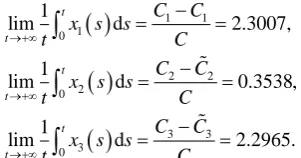
1 1

1 0

2 2

2 0

3 3

3 0

1

lim d 2.3007,

1

lim d 0.3538,

1

lim d 2.2965.

t t

C C

x s s

t C

C C

x s s

t C

C C

x s s

t C

→+∞

−

= =

−

= =

−

= =

∫



see Figure 1, which is obtained by applying the Milstein method [25].

Figure 1 shows the simulations of the solutions of systems (SM), besides,

( ) ( )

1 , 2

x t x t and x t3

( )

are shown in Figure 1. We see that x t1

( ) ( ) ( )

,x2 t ,x t3

tend to constants, which is consistent with the results of Theorem 4.1. the solu-tions of systems (SM) fluctuate around a small zone. Thus, we think the system (SM) is permanent.

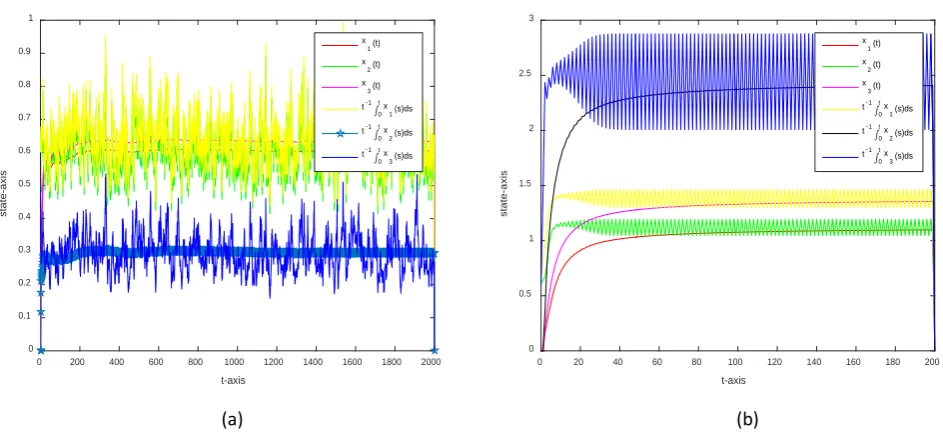
Since the parameters given above meet the hypothesis 2: c11>c12+c13,

22 21 23

c >c +c _and c33>c31+c32. According to Theorem 5.1, we can get the

system (SM) is global attractively, see Figure 2.

Figure 2 shows the simulations of the solutions of systems (SM), From Figure 2(a) and Figure 2(b), we can see that the solution of the system is globally at-tractively, whether with or without random perturbations.

7. Conclusions and Discussions

[image:15.595.297.448.404.483.2]