In the shadows of giants : a tomographic method for analysing the orbits of transiting exoplanets

IN THE SHADOWS OF GIANTS: A TOMOGRAPHIC METHOD

FOR ANALYSING THE ORBITS OF TRANSITING

EXOPLANETS

Grant Robert MacKinnon Miller

A Thesis Submitted for the Degree of PhD

at the

University of St Andrews

2013

Full metadata for this item is available in

Research@StAndrews:FullText

at:

http://research-repository.st-andrews.ac.uk/

In the Shadows of Giants

A tomographic method for analysing the orbits of transiting exoplanets

by

Grant Robert MacKinnon Miller

Submitted for the degree of Doctor of Philosophy in Astrophysics

Declaration

I, Grant Robert MacKinnon Miller, hereby certify that this thesis, which is approximately 30,000 words in length, has been written by me, that it is the record of work carried out by me and that it has not been submitted in any previous application for a higher degree.

Date Signature of candidate

I was admitted as a research student in September 2008 and as a candidate for the degree of PhD in September 2008; the higher study for which this is a record was carried out in the University of St Andrews between 2008 and 2012.

Date Signature of candidate

I hereby certify that the candidate has fulfilled the conditions of the Resolution and Regula-tions appropriate for the degree of PhD in the University of St Andrews and that the candidate is qualified to submit this thesis in application for that degree.

Copyright Agreement

In submitting this thesis to the University of St Andrews we understand that we are giving permission for it to be made available for use in accordance with the regulations of the Uni-versity Library for the time being in force, subject to any copyright vested in the work not being affected thereby. We also understand that the title and the abstract will be published, and that a copy of the work may be made and supplied to any bona fide library or research worker, that my thesis will be electronically accessible for personal or research use unless ex-empt by award of an embargo as requested below, and that the library has the right to migrate my thesis into new electronic forms as required to ensure continued access to the thesis. We have obtained any third-party copyright permissions that may be required in order to allow such access and migration, or have requested the appropriate embargo below.

The following is an agreed request by candidate and supervisor regarding the electronic publication of this thesis: Access to Printed copy and electronic publication of thesis through the University of St Andrews.

Date Signature of candidate

Abstract

The radial velocity anomaly which affects spectroscopic observations of stars undergoing tran-sit by a companion body is known as the Rostran-siter-McLaughlin effect. This effect can be used to measure the obliquities of the orbits of transiting planets. In this thesis I present a tomo-graphic method for analysing the effect, which manifests itself in stellar spectral line-profiles. I implement this method on seven systems known to host transiting planets, and some sys-tems with early-type host stars, for which the transit events have not yet been shown to be the result of planetary companions.

Despite being well-suited to examining systems with early-type, rapidly-rotating host stars which have a more pronounced Rossiter-McLaughlin effect, I find the tomographic method is able to produce reasonable results for the system parameters of planets orbiting relatively slowly-rotating stars. I show that the method provides a significant increase in the accuracy of determinations of the stellar rotation rate and is able to better constrain values for the transit impact parameter.

Acknowledgements

Firstly I would like to thank my supervisor Professor Andrew Collier Cameron for his help and advice on all matters over the past few years. His infectious enthusiasm for the field of astrophysics has been an inspiration to me. Thanks to Rim for helping me with the reduction of my data and to David for being a cracking office-mate and for producing some lovely plots for me.

Next I extend my gratitude to all the others in the astronomy department at the University of St Andrews who have made my time here so enjoyable. Special thanks have to go to my colleague and good friend Lee Kelvin, with whom I’ve had many a lively debate and quite a few "great ideas", David Hill, Alex and Noé for taking me under their wings when I started and introducing me to the next level of quizzing, Aaron for his many intriguing puzzles, interesting facts, and for providing me with an evenly matched pool opponent, Paul for his regular IT support, for giving me someone to talk to/at about my favourite TV shows, and for the regular jump-starts he had to give my car (thanks also to John for this), Joe for being a wonderful friend during the final part of my PhD and for reminding me to try and always wear a smile and to "man-up", and last but not least, Craig and Neil for their good advice and reassuring words during the final parts of my write-up.

A huge thank you to Jack and Kelly for giving me a place to (try and) sleep while finishing this thesis thesis.

Thanks to my highschool physics teacher Mrs Montgomery for inspiring me to study astro-physics, and to all the staff and students at the University of Glasgow who helped me attain my undergraduate degree.

Thank you to Meg for allowing me to play "soccer" for her team, but more importantly for being my closest friend over the last year, reminding me that it is important to work hard in order to play hard once the work is done, and finally, for proof-reading this thesis!

“This space we declare to be infinite, since neither reason, convenience, possibility,

sense-perception nor nature assign to it a limit. In it are an infinity of worlds of the

same kind as our own.”

Contents

Declaration i

Copyright Agreement iii

Abstract v

Acknowledgements vii

1 Introduction 1

1.1 A brief history . . . 1

1.2 Methods for detecting exoplanets . . . 2

1.2.1 The radial velocity method . . . 2

1.2.2 Gravitational microlensing . . . 3

1.2.3 Astrometry . . . 6

1.2.4 Pulse timing . . . 6

1.2.5 Transit-timing variations . . . 6

1.2.6 Direct imaging . . . 7

1.2.7 The transit method . . . 8

1.2.8 Other possible methods for exoplanet detection . . . 15

1.3 The SuperWASP Project . . . 15

1.3.1 The Telescopes . . . 17

1.3.2 Data Pipeline and Archive . . . 17

1.3.3 The WASP Planets . . . 19

1.3.4 Follow-up observations . . . 19

1.4 Planet formation and orbital evolution . . . 20

1.5 The Rossiter-McLaughlin Effect . . . 22

2.1 Introduction . . . 28

2.2 Methods for analysing the Rossiter-McLaughlin effect . . . 28

2.3 A new tomographic method for analysing the Rossiter-McLaughlin effect . . . 30

2.3.1 Fitting the model . . . 33

2.3.2 Markov chain Monte Carlo technique . . . 34

2.3.3 Implementation of the new method . . . 35

3 A case study: WASP-3b 37 3.1 Introduction . . . 38

3.2 Observations and analysis . . . 39

3.2.1 Photometric and spectroscopic datasets . . . 39

3.3 Results . . . 43

3.3.1 Age from evolutionary tracks . . . 44

3.3.2 Age from gyrochronology . . . 47

3.4 Conclusions . . . 47

4 Rossiter-McLaughlin analyses of five transiting systems 51 4.1 Introduction . . . 52

4.2 . . . 52

4.2.1 Photometry . . . 53

4.2.2 Spectroscopy . . . 53

4.2.3 WASP-16b . . . 53

4.2.4 WASP-17b . . . 54

4.2.5 WASP-18b . . . 54

4.2.6 WASP-23b . . . 54

4.2.7 WASP-31b . . . 54

4.3 Results . . . 54

4.3.1 WASP-16b . . . 54

4.3.2 WASP-17b . . . 59

4.3.3 WASP-18b . . . 59

4.3.4 WASP-23b . . . 66

4.5 Conclusions . . . 75

5 Detecting planets orbiting early-type stars 81 5.1 Introduction . . . 82

5.2 Target selection . . . 82

5.3 Observations . . . 83

5.4 Results . . . 83

5.4.1 J025712 . . . 83

5.4.2 J091603 . . . 86

5.4.3 J205027 . . . 87

5.4.4 J212530 . . . 91

5.4.5 Ephemeris drift . . . 91

5.5 Preliminary tomographic MCMC analysis . . . 93

5.6 Other selected targets . . . 93

5.7 Conclusions . . . 93

6 Conclusions and Outlook 97 6.1 Main findings . . . 98

6.1.1 Moderately fast-rotating stars . . . 98

6.1.2 Slowly rotating stars . . . 98

6.1.3 Early-type stars . . . 99

6.1.4 Orbital obliquities and the migration process . . . 100

6.2 Outlook . . . 101

A SuperWASP follow-up observations using the James Gregory Telescope 103

Online resources 107

Images in chapter headings 109

List of Figures

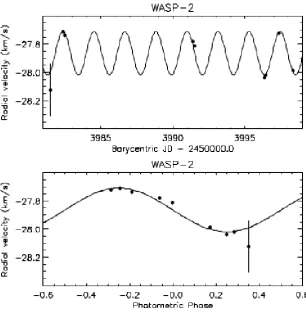
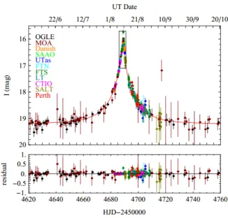
1.1 Plot of the radial velocity data for WASP-2b. The top panel shows the data over multiple orbits and the bottom panel shows the phase-folded plot. Plot taken from Collier Cameron et al. (2007a). . . . 4 1.2 A lightcurve for object showing the increase in brightness observed by mutiple

telescopes as the lens stars passes in front of the background star. Plot taken from Bozza et al. (2012) . . . 5 1.3 Direct imaging of the four planets discovered orbiting HR 8799. Image from

Marois et al. (2010). . . . 7 1.4 The top panel shows a lightcurve with uncorrelated ("white noise") only. The

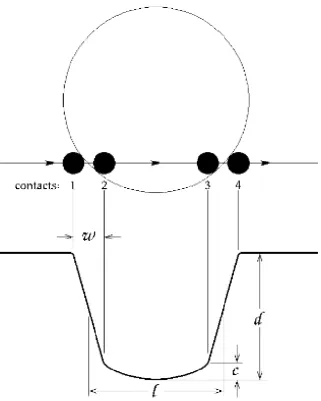
middle panel shows red noise only. The bottom panel shows the result of com-bining the red and white noise. The bottom lightcurve has features which resemble transit lightcurves produced from high precision, wide-field surveys. (Pont et al., 2006). . . 10 1.5 Schematic of an ideal transit lightcurve from Brown et al. (2001). . . . 12 1.6 Lightcurve of HD 209458 taken with the STIS spectrograph on the Hubble Space

Telescope (Brown et al., 2001). . . . 14 1.7 Plot of mass vs semi-major axis for all planets discovered as of December 2011.

Exoplanets discovered via the transit method are denoted by blue circles, radial velocity method by black wedges, microlensing by red stars, timing by grey squares, and direct imaging by orange triangles. Plot courtesy of Keith Horne (http:// star-www.st-and.ac.uk/kdh1). . . . 16 1.8 The SuperWASP-North assembly on the island of La Palma (from www.superwasp.org/). 18 1.9 The top lightcurve was taken using the 60 cm telescope at Keele University. The

middle two lightcurves were taken by the author using the James Gregory Telescope at St Andrews, and the bottom lightcurve was taken using KeplerCam on the 1.2 m telescope at the Fred Lawrence Whipple Observatory in Arizona. The figure is taken from the discovery paper Alsubai et al. (2011). . . . 20 1.10 The RM waveforms for three different planet trajectories. Notice all three have

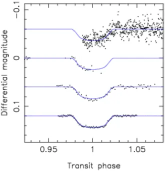
identical impact parameter so therefore would have identical photometric transit signatures. The solid lines include the effect of limb darkening (Gaudi & Winn, 2007). . . . 24 1.11 Top: Phase-folded WASP data for planet WASP-13b. Middle: JGT data for the

2.1 Diagram showing the various co-ordinates involved in modeling the RM effect. x_p and zpare the co-ordinates of the planet on the plane of the sky, upis the projected distance of the planet from the stellar rotation axis, b is the impact parameter of the transit, andλis the projected angle between the stellar rotation axis and the orbital axis of the planet. Diagram courtesy of Andrew Collier Cameron. . . . 32

3.1 Upper panel: Phase-folded plot of the 6 out-of-transit radial velocity mea-surements which are not affected by any time-varying asymmetry of the line-profile. The out-of-transit RV fit was calculated by adjusting the velocity semi-amplitude, orbital eccentricity, argument of periastron and true anomaly. The position of the planet over the stellar disc, ratio of star/planet radii, impact parameter and non-linear limb darkening coefficients were used to model the RM anomaly during transit. Lower panel: Phase-folded plot of all 8 sets of photometric data analysed in this study. . . 40

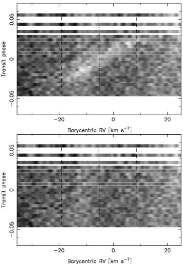
3.2 Top: Residual map of time series CCFs with the model spectrum subtracted leaving the bright time-variable feature due to the light blocked by the planet.

Bottom: Here the best-fit model for the time-variable feature has also been removed to show the overall residual. The horizontal dotted line marks the phase and radial-velocity of mid-transit. The shift of this line from zero shows the underlying systemic radial-velocity. The two vertical dashed lines are at

±vsinI from the systemic radial velocity (marked by the vertical dotted line). The crosses on the vertical dotted line denote the two points of contact at both ingress and egress. . . 41

3.3 Correlation plots for the four parameters calculated from the RM effect. The distribution of points shows each accepted step on the Markov chain. . . 45

3.4 The new position of WASP-3 in the T_{e f f} vs R/M1/3 plane. The larger of the two boxes shows the data from the discovery paper. The smaller box shows the error range from this study. The lines show evolutionary tracks from Girardi et al. (2000) for 1.2, 1.3 and 1.4 solar masses and isochrones at 0.1, 0.5, 1, 1.5, 2, 2.5 and 3 billion years. The tracks and isochrones here are for stars with solar metallicity,[M/H] =0. . . 46

deter-4.1 Top: Residual map of WASP-16 time series CCFs with the model average line profile subtracted. Despite the slow rotation rate of the star, a noticeable time-variable feature is still left behind due to the light blocked by the planet. Bot-tom: Here the best-fit model for the time-variable feature has also been re-moved to show the overall residual. The horizontal dotted line marks the phase of mid-transit. The shift of the vertical dotted line from zero shows the under-lying systemic radial velocity. The two vertical dashed lines are at±vsinI from the systemic radial velocity. The crosses on the vertical dotted line denote the two points of contact at both ingress and egress. The light and dark vertical features arise due to crosstalk between overlapping spectral lines in the wings of the CCF. . . 57 4.2 Modified Hertzprung-Russell diagram showing the updated position of

WASP-16 in the density-effective temperature plane. The isochrones for the ages 0.1, 0.6, 1, 2, 3, 4, 5, 6, 7, 8, 9 and 10 Gyr (left to right, shown by black curves) and the evolutionary mass tracks for masses 0.9, 1.0, 1.1 and 1.2M(right to left, red dashed lines) are from Demarque et al. (2004) who used Yonsei-Yale models. . . 58 4.3 For WASP-17 the planet signature moves from the blue-shifted side of the line

profile to the red-shifted side. This is a clear indication that the planet is in a retrograde orbit around the star. The significance of the top and bottom panels and an explantion of the markings is given in the caption for Figure 4.1. . . 61 4.4 Modified Hertzprung-Russell diagram showing the updated position of

WASP-17 in the density-effective temperature plane. The isochrones for the ages 0.1, 0.6, 1, 2, 3, 4 and 5 Gyr (left to right, black curves) and the evolutionary mass tracks for masses 1.1, 1.2, 1.3 and 1.4M(right to left, red dashed lines) are from Demarque et al. (2004). . . 62 4.5 In the case of WASP-18 the faster rotation rate produces a clearly resolved

bright planet signature moving in a prograde direction. The plot shows the sig-nature starting and finishing near the maximumvsinIvalue. This suggests the planet is in a well-aligned orbit with a low impact parameter. The significance of the top and bottom panels and an explantion of the markings is given in the caption for Figure 4.1. . . 64 4.6 Modified Hertzprung-Russell diagram showing the updated position of

WASP-18 in the density-effective temperature plane. The isochrones for the ages 0.1, 0.5, 1, 2, 3, 4, and 5 Gyr (left to right, black curves) and the evolutionary mass tracks for masses 1.1, 1.2, 1.3 and 1.4M(right to left, red dashed lines) are from (Demarque et al., 2004). . . 65 4.7 Correlation plots of the MCMC output from our analysis of WASP-23. . . 68 4.8 Correlation plot of the MCMC output from the analysis of WASP-23 by Triaud

et al. (2011) with no prior set on vsinI. Triaud et al. (2011) useβ to denote projected spin-orbit misalignment angle as opposed toλ. . . 69 4.9 Correlation plot of the MCMC output from the analysis of WASP-23 by Triaud

4.10Top: The anomaly is clearly visible in the upper plot despite the slow rotation rate of WASP-23. It appears to move from the red to the blue side of the line profile as the transit occurs. This simple piece of informations helps break the ambiguity over the system’s alignment, showing that it is indeed in a prograde orbit. The significance of the top and bottom panels and an explantion of the markings is given in the caption for Figure 4.1. . . 70 4.11 Modified Hertzprung-Russell diagram showing the updated position of

WASP-23 in the density-effective temperature plane. The isochrones for the ages 6-20 Gyr (left to right, black curves) and the evolutionary mass tracks are from (Demarque et al., 2004). . . 71 4.12Top: The trailed spectra for WASP-31b, showing a clear anomaly moving in

the prograde direction. The significance of the top and bottom panels and an explantion of the markings is given in the caption for Figure 4.1. . . 73 4.13 Modified Hertzprung-Russell diagram showing the updated position of

WASP-31 in the density-effective temperature plane. The isochrones for the ages 0.1, 0.8, 1, 2, 3, 4, 5, 6, 7, 8, 9 and 10 Gyr and the evolutionary mass tracks are from (Demarque et al., 2004). . . 74 4.14 Plot showing the magnitude of the projected spin-orbit misalignment angle

against stellar effective temperature. On the plot WASP-16=blue circle, WASP-17 = blue square, WASP-18= blue triangle, WASP-23 = blue diamond and WASP-31 = blue star. The plot shows the tendancy of systems with effective temperature greater than 6250 K to be misaligned. However our values for WASP-18 show it to be an exception to this trend. The vertical dotted line is at 6250 K and corresponds to the temperature above which stars no longer have a convective outer shell. The horizontal dotted line is atλ=30◦. Systems above this line as considered to be significantly misaligned. . . 78 4.15 The intrinsic spectral linewidth, vg, plotted as a function of stellar effective

temperature,T_{e f f}. The linear trend gives an empirical calibration of the degree of turbulence as a function of T_{e f f}. . . 79 5.1 Top: Trailed spectra of the 29 observations made of J025712. Barycentric radial

velocity is plotted along the x-axis and the y-axis shows the orbital phase at which each observation was taken (where zero phase corresponds to predicted mid-transit time). Flux is plotted as a greyscale, with black indicating lower flux and white higher flux. The darker region shows the core of the line-profile.

Bottom: Here the average of all the spectra has been subtracted from each observation, showing the broad, bright signature of the transiting stellar-mass companion. . . 85 5.2 The average line-profiles of the initial and final observations of J025712. The

5.3 Top: Trailed spectra of the 25 observations of J025712. Bottom: Here the average of all the spectra has been subtracted from each observation, revealing the broad tiger-stripe pattern created by non-radial stellar pulsations. . . 88 5.4 Top: As in Figure 5.3, all 25 spectra stacked. Bottom: A streak caused by

non-radial pulsations on the stellar surface can be seen once the average of the spectra has been removed. . . 89 5.5 Top: Trailed spectra map of the 22 observations of J205027. Bottom: With the

average line profile subtracted, no obvious residual signature is revealed via this preliminary analysis. . . 90 5.6 Top: Trailed spectra of the 10 observations of J212530.Bottom: After removing

the average spectrum there is no immediate signature of a transiting companion. 92 A.1 Plots output from the JGT data reduction pipeline for the observations of the planet

Qatar-1b. The data shown here helped confirm the planet-sized radius of the transiting object (Alsubai et al., 2011). . . . 105 A.2 A blended eclipsing binary system. Here the JGT observations have revealed that

List of Tables

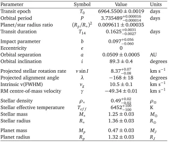
3.1 Results of MCMC analysis compared to those presented in the literature. . . 42 3.2 Values for projected stellar rotation rate, spin-orbit misalignment angle and

width of the intrinsic stellar line profile compared to those from the two pre-vious Rossiter-McLaughlin studies of WASP-3b. Note: The value obtained for

vsinI through spectral analysis is 13.4±1.5 km s−1(Pollacco et al., 2008). . . 43 4.1 System parameters from the MCMC analysis for WASP-16b. . . 56 4.2 Age and mass values for WASP-16 from comparison with various isochrone

models. . . 56 4.3 System parameters from the MCMC analysis for WASP-17. . . 60 4.4 Age and mass values for WASP-17 from comparison with various isochrone

models. . . 60 4.5 System parameters from the MCMC analysis for WASP-18. . . 63 4.6 Age and mass values for WASP-18 from comparison with various isochrone

models. . . 65 4.7 System parameters from the MCMC analysis for WASP-23. . . 67 4.8 System parameters from the MCMC analysis for WASP-31. . . 72 4.9 Age and mass values for WASP-31 from comparison with various isochrone

models. . . 72 4.10 Comparison of vsinI values obtained via different methods (Sytems measured

in this chapter are marked with *). . . 77 5.1 Properties of the target stars and a log of the observations. . . 84 5.2 The uncertainties on the predicted transit time for each target, calculated from

1

Introduction

1.1

A brief history

Chapter 1. Introduction

1995, that the first planet orbiting a Main Sequence star (similar to our Sun) was discovered (Mayor & Queloz, 1995).

Since then, the discovery rate of exoplanets has increased exponentially. There have been over one hundred ground and space-based planet-search projects (many still operating and some proposed for the future) utilising several different scientific methods in order to confirm the detection of planets orbiting distant stars. To date over 800 exoplanets have been dis-covered, with a wide range of masses, residing in almost 700 planetary systems, all (so far) within our own galaxy1.

The driving aims of the search for exoplanets are learning about the distribution of plane-tary characteristics in our galaxy (is our planet, or indeed Solar System typical or a relatively unusual configuration?), refining our models of how planets and planetary systems form and evolve, and the ever-intriguing possibility of discovering small, Earth-like planets around main sequence stars capable of harbouring life.

1.2

Methods for detecting exoplanets

There are a number of different scientific methods that can be implemented in order to detect and confirm the existence of exoplanets. Most of these techniques involve observing the effect the planet has on its host star, as the planet is too small and faint (compared to its nearby star) to be resolved directly with current instruments. Each method has its own advantages and disadvantages, and sensitivity to different regions of the planet parameter space. The following is an overview of each of the detection methods which have been successfully im-plemented in the search for exoplanets to date.

1.2.1

The radial velocity method

1.2. Methods for detecting exoplanets

stellar spectrum due to the changing radial velocity of the star. The stellar wobble is caused by the gravitational pull of an orbiting planet. The more massive the planet the larger the radial-velocity shift. The Doppler shift of the light in the stellar spectrum is usually measured by taking an average of the star’s spectral lines and measuring how the centroid of this aver-age line profile moves over a period of time. The shifting spectrum gives information on the period of the planet’s orbit and a lower limit for the mass of the planet. The true mass cannot be found using this method alone, as the inclination,i, of the planet’s orbital axis to our line-of-sight is not known. Therefore the planet masses derived from radial velocity measurements are always stated asM_Psini.

At the moment the radial velocity method is by far the most productive method for covering extrasolar planets, with over half of the known extrasolar planets having been dis-covered from radial velocity measurements alone. The radial velocity method is well suited to detecting large planets around relatively nearby stars, as the brighter the star and the larger the Doppler shift the easier it is to measure. Younger hot stars earlier than around F5 on the main sequence pose a problem for radial velocity searches due to their lack of spectral lines and increased chance of rotational broadening.

The amplitude of the stellar radial velocity variation, K_∗, is related to the mass of the orbiting companion by the equation:

K_∗= 2πaMPsini (M_P+M_∗)Pp1−e2

(1.1)

whereais the orbital semi-major axis,Pis the period of orbit andeis the orbital eccentricity. Therefore by estimatingM_∗from the spectral type and assuming a circular orbit andM_∗M_P,

M_Psinican be measured directly from the maximum radial velocity shift.

Figure 1.1 shows an example of the sinusoidal curve that is produced from radial velocity measurements. This particular set of data was used to confirm the existence of the planet WASP-2b (Collier Cameron et al., 2007a).

1.2.2

Gravitational microlensing

Chapter 1. Introduction

Figure 1.1: Plot of the radial velocity data for WASP-2b. The top panel shows the data over multiple

1.2. Methods for detecting exoplanets

microlensing. If the foreground star (known as the ’lens star’) has a planet orbiting it there is a chance that its gravitational field may cause a noticeable addition to the microlensing event (Gould & Loeb, 1992). This method allows good measurement of the mass of the planet and is also capable of detecting low mass Earth-like planets (Beaulieu et al., 2006). One major disadvantage of microlensing as a planet searching method is that observations of each object can only be performed once, as it relies on the chance alignment of two stars separated by a large distance. This means there is no possibility of follow-up observations and all the analysis has to be done on one single event. However, gravitational microlensing is capable of detect-ing planets at much larger distances than the other detection methods which are limited to bright, nearby stars. It can be used to discover small planets as far away as the galactic bulge and is the only method capable of detecting free-floating planets (Gaudi et al., 2009).

Figure 1.2: A lightcurve for object showing the increase in brightness observed by mutiple telescopes as

Chapter 1. Introduction

1.2.3

Astrometry

Similar to the radial velocity method, astrometry involves observing the effect of the grav-itational pull of a planet on its host star. Instead of dealing with the Doppler shift of the spectrum the astrometry method involves accurately measuring the position on the sky of the host star as a function of time (Combrinck, 1983). To date this method has not been used to detect any previously undiscovered extrasolar planets, however it has been used at least once to measure the mass of a known extrasolar planet (Benedict et al., 2002). Progress will be made in the field of astrometry with the launch of the Gaia mission in 2013 (Cacciari, 2009) and the proposed Near Earth Astrometric Telescope (NEAT) mission (Malbet et al., 2012).

1.2.4

Pulse timing

The period of a pulsar can be measured to an extremely high level of accuracy (Kaspi, 1995). Planets can be detected around pulsars due to the changes in arrival time of the pulses they cause via their gravitational pull on the pulsar (Wolszczan & Frail, 1992). The level of ac-curacy possible with pulsar timing means it is a good method for finding low mass planets, however it is often overlooked as it does not involve main sequence stars.

1.2.5

Transit-timing variations

1.2. Methods for detecting exoplanets

1.2.6

Direct imaging

As mentioned in the introduction to this section, direct imaging of extrasolar planets is very difficult as they are extremely faint compared to their host stars. This means that so far detections have been restricted to massive Jupiter-like planets at large distances from their host stars (tens or even hundreds of AU). The first proposed image of an extrasolar planet was announced in 2004 (Chauvin et al., 2004). Since then there have been a handful of successful attempts (Marois et al., 2008; Kalas et al., 2008; Neuhäuser & Schmidt, 2012). Figure 1.3 from Marois et al. (2008) shows the high-contrast near infrared imaging of 4 planets orbiting HR 8799. As only the radius of the planet and not the mass can be estimated from this method there is often debate as to whether these large stellar companions are actually brown dwarfs.

Figure 1.3: Direct imaging of the four planets discovered orbiting HR 8799. Image from Marois et al.

Chapter 1. Introduction

1.2.7

The transit method

This method involves photometrically measuring the drop-off in brightness observed when a planet crosses the stellar photosphere of its host star and blocks a small portion of the emitted light as seen from the Earth’s viewpoint, just as occasionally happens with the transits of Venus and Mercury in our own solar system (Deeg, 1998). Even for a large, Jupiter-sized planet the dip in brightness is still only very small (∼1%). The radius of the eclipsing object can be estimated from the magnitude of the dip in light. Photometric transit observations also provide information on the inclination of the planet’s orbit, therefore combining transit observations with radial velocity measurements is an ideal way to reveal the true mass and density of the planet. One disadvantage of this method is that only a small fraction of stars have planets orbiting at inclinations that would cause a transit event as seen from Earth. The fraction also decreases as a function of the planet’s distance from its host star. The probability of a planet’s orbit being aligned so that it is seen to transit decreases as a function of its orbital separation from its host star (Horne, 2003):

P_t≈R_∗/a, (1.2) whereR_∗is the stellar radius andais the orbital semi-major axis of the planet. Therefore if it were our Solar System being observed, the probability of the Earth transiting the Sun would be roughly 0.5%. For Jupiter, even though it is much larger than the Earth, the probability drops to 0.1% due to its larger separation from the Sun. Larger planets cause greater dips in the brightness of their host star making them easier to detect compared to small, Earth-like planets. There is also more chance of detecting a planet with a short orbital period (_∼1₋5 days) as the fraction of time it spends in-transit is higher and multiple transit observations can be made in a short space of time. Putting all of these factors into consideration it becomes clear that transit surveys are very good at finding large, gas-giant planets which orbit very close to their host stars (<0.1AU) with short orbital periods. These planets are known as ‘hot Jupiters’ due to their physical similarity to our planet Jupiter and their close proximity to their stars.

1.2. Methods for detecting exoplanets

the mass of the transiting object. These wide-field, ground-based transit surveys have major difficulties detecting smaller, Earth-like planets, which exist in the habitable zone around their star, with orbital separations 10₋100 greater than those of hot Jupiters. This is due to their long periods, minute transit depths (˜0.1%) and low probability that the inclination of the sys-tem allows their transits to be visible from Earth.

Chapter 1. Introduction

Figure 1.4: The top panel shows a lightcurve with uncorrelated ("white noise") only. The middle

1.2. Methods for detecting exoplanets

There are many system parameters which can be measured through photometric observa-tions of the star. Kepler’s third law means that by measuring the period P of the transiting planet (i.e. the interval between successive transits), and estimating the stellar massM_∗from its spectral type, one can calculate a value for the orbital separation of the planet,a:

a3= G(M∗+MP)

4π2 P

2_{, (1.3)}

whereM_P can be neglected if we assume that M_∗M_P.

Values for other system parameters can be gained by analysing the shape of the tran-sit lightcurve, which is a plot of how a target star’s brightness drops as a planet passes in front of its disc. It is the characteristics of the transit lightcurve (width, depth, duration of ingress/egress) that are the key to determining the major parameters of the system such as the radius of the planetRP, the orbital inclination iand the impact parameter (how close to

the centre of the stellar disc the transiting object crosses)b.

Figure 1.5 shows the measurable components of a transit lightcurve. The transit duration

l, the ingress and egress duration w, the transit depth d and the central curvature C. The reason that the transit lightcurve is not exactly box-shaped and rather has sloped edges and a curved base is due to stellar limb-darkening. The stellar radius can be calculated from the transit durationl, impact parameter band transit depthdusing the relation

R_∗ a =

l P

π

(1+pd)2−b2, (1.4)

where the impact parameterbis a value between 0 and 1 representing how close to the centre of the stellar disc the planet is during mid transit (Collier Cameron et al., 2007b). It is related to the orbital inclination via the relation b= acos_Ri

∗. Neglecting limb darkening, Seager &

Mallén-Ornelas (2003) show that the transit depthd provides an estimate for the radius ratio of the star and planet:

d≡ Fout of transit−Fin transit

F_{out of transit} . (1.5)

Chapter 1. Introduction

1.2. Methods for detecting exoplanets

d= A∗−(A∗−AP)

A_∗ =

AP

A_∗, (1.6)

and substituting in the radii of the star and planet we get

d= πR

2 P πR2_∗ =

_R P R_∗

2

. (1.7)

Chapter 1. Introduction

Figure 1.6: Lightcurve of HD 209458 taken with the STIS spectrograph on the Hubble Space Telescope

(Brown et al., 2001).

The first successful detection of an extrasolar planet using the transit method was made by Charbonneau et al. (2000). They observed two transits of HD 209458b for which radial veloc-ity variations had already been reported by Henry et al. (1999). The observations were taken using the STARE project’s (Brown & Charbonneau, 1999) Schmidt camera which has a 6◦ field-of-view and a 2048x2048 pixel CCD. The observations suggested values RP =1.27±0.02RJ

for the radius of the planet and i=87.1◦±0.2◦for the inclination of its orbit to the line-of-sight. Using the results from the previous radial-velocity measurements combined with their value for the orbital inclination, Charbonneau et al. calculated a value for the planet’s mass ofMP =0.63MJ. Using the values for the radius and mass of the planet they were also able to

calculate its average density, surface gravity and escape velocity. A high-precision photomet-ric lightcurve of HD 209458 taken using the Hubble Space Telescope can be seen in Figure 1.6.

1.3. The SuperWASP Project

Udalski et al., 2003; Bakos et al., 2009; McCullough et al., 2005; Pollacco et al., 2006c) and the space-based COROT (Baglin et al., 2002) and Kepler (Borucki et al., 2010) missions.

The work in this thesis is based on observations of planets and planet candidates detected through the SuperWASP project. In the following section the project, its goals and success will be outlined.

1.2.8

Other possible methods for exoplanet detection

Other detection methods which have been proposed include using a polarimeter to detect the polarized light that the planet is reflecting, looking for features in circumstellar discs which are caused by the presence of planets and measuring light variations caused by the changing orbital phase of a planet.

A plot showing mass vs semi-major axis for all exoplanets discovered by all the methods described above can be seen in Figure 1.7. It nicely highlights which regions of the parameter space each detection technique is sensitive to.

1.3

The SuperWASP Project

The SuperWASP (Super Wide Angle Search for Planets (Pollacco et al., 2006a) project is the world’s leading ground-based search for transiting extrasolar planets. It is operated by eight academic institutions in the UK and the Canary Islands, namely: Queens University Belfast, the University of St Andrews, Keele University, the University of Leicester, the Isaac Newton Group of telescopes, the University of Cambridge, the Open University and the Instituto de As-trofisica de Canarias. It involves two remotely operated observatories, one in each hemisphere so as to observe the whole sky. SuperWASP-North, which experienced first light in 2004, is located amongst the Isaac Newton Group of telescopes at the Observatorio del Roque de los Muchachos on the island of La Palma in the Canary Islands. SuperWASP-South is located at the South African Astronomical Observatory station in Sutherland, South Africa and made its first observations in 2006.

Chapter 1. Introduction

Figure 1.7: Plot of mass vs semi-major axis for all planets discovered as of December 2011. Exoplanets

1.3. The SuperWASP Project

the transit of the known planet HD 209458 (Kane et al., 2004).

1.3.1

The Telescopes

Each observatory consists of a robotic equatorial fork mount which holds 8 Canon 200mm f/1.8 lenses backed with high quality 2048x2048 pixel CCDs (see Figure 1.8). The entire assembly is housed in a small enclosure with a retractable roof. The opening/closing of the roof, pointing of the cameras and data taking are all fully automated. Each camera has a 7.8o_×7.8ofield-of-view meaning the total FOV is almost 500 square degrees (30 degrees in declination by 1 hour in right ascension (Pollacco et al., 2006a). Initially the set-up did not include any optical filters, however infrared blocking filters, which allow light in the range 400nm - 700nm to be transmitted, were installed on both the northern and southern facilities before the start of regular operations in early 2006.

1.3.2

Data Pipeline and Archive

Chapter 1. Introduction

1.3. The SuperWASP Project

the data.

1.3.3

The WASP Planets

SuperWASP detected its first planet (WASP-1b) in 2006 (Cameron et al., 2007). WASP-1b is a hot Jupiter with a radius of 1.33₋2.53R_J and a mass of 0.80₋0.98M_J. It was first detected as a photometric transit in the 2004 season of SuperWASP data and was later confirmed as a planet using the SOPHIE spectrograph at the Observatoire de Haute-Provence. Since then the SuperWASP project has become the most successful ground-based transiting planet survey and has discovered over 80 transiting extrasolar planets to date3. The planets discovered by the survey are all hot gas-giants, ranging from the Saturn-sized WASP-29b to the 10M_J planet WASP-18b.

1.3.4

Follow-up observations

The SuperWASP project also performs follow-up photometry and radial velocity measure-ments using several telescopes in different locations around the world. These follow-ups are performed on the best candidates, from the initial photometric observations from the WASP cameras, to confirm whether or not a planet is causing the observed brightness variation. There are many telescopes across the globe which are used to perform follow-up observations of candidates first detected in the data from La Palma and Sutherland. The main instruments used for radial velocity follow-up observations are the Coralie spectrograph (R=50, 000) on the 1.2 m Swiss Euler Telescope at La Silla in Chile, and the Sophie spectrograph (R=75, 000) on the 1.93 m telescope at Haute-Provence Observatory in the south of France. Multiple tele-scopes are used to perform photometric follow-up observations of SuperWASP targets, includ-ing the UK’s largest optical telescope, the 1 m James Gregory Telescope (JGT) housed at the University of St Andrews observatory.

During the course of my doctorate degree I have spent over one hundred nights observing on the JGT, the results of which have lead to the rejection of multiple SuperWASP candidates as astrophysical false-positives, and I have also helped in the confirmation of multiple WASP planets. Figure 1.9 shows a comparison of follow-up photometery of the planet Qatar-1b (the first planet announced by the Qatar Exoplanet Survey, QES (Alsubai et al., 2011)) from 3 ground-based telescopes at different locations in the northern hemisphere. The data for

Chapter 1. Introduction

the two curves in the middle of this figure were taken by myself from the JGT and were subsequently used to confirm that the transiting companion was of planetary radius.

I have also been on one radial velocity follow-up run on the Nordic Optical Telescope (NOT) located at the Roque de los Muchachos Observatory on La Palma in the Canary Islands, and two separate observing runs on the 1.93-m telescope at the Haute-Provence Observatory. The data taken from these runs has lead to the mass confirmation of multiple WASP planets.

Figure 1.9: The top lightcurve was taken using the 60 cm telescope at Keele University. The middle two

lightcurves were taken by the author using the James Gregory Telescope at St Andrews, and the bottom lightcurve was taken using KeplerCam on the 1.2 m telescope at the Fred Lawrence Whipple Observatory in Arizona. The figure is taken from the discovery paper Alsubai et al. (2011).

1.4

Planet formation and orbital evolution

1.4. Planet formation and orbital evolution

Solar System. It can be shown that in the core-accretion scenario of gas giant formation (Pol-lack et al., 1996), which is currently the most widely accepted formation model, these planets must form beyond a certain distance from their host star known as the ’snow line’, where tem-peratures are low enough (∼150 K) for ice to form on dust grains therefore allowing them to clump together (Sasselov & Lecar, 2000). This point occurs around 4 AU from a Sun-like star. The existence of gas giants at orbital separations smaller than 0.1 AU therefore means that instead of forming in-situ they must migrate inwards through the system towards their host stars after they form. There is no clear consensus on how these planets undergo migration, however there are a few leading theories. The inital view of planet migration involves the planet undergoing gravitational interactions with a protoplanetary disc causing the planet to lose angular momentum and move inwards through the disc (Goldreich & Tremaine, 1980). Assuming the protoplanetary disc is aligned with the stellar spin axis, this process would lead to planets in well-aligned orbits around the equator of their host star. However, there have more recently been several observations of planets confirmed to be on highly misaligned orbits (Triaud et al., 2010; Albrecht et al., 2012a; Anderson et al., 2010). This has lead to processes such as planet-planet scattering and the Kozai mechanism with tidal dampening being viewed as the most likely methods for transporting gas giant planets inwards through their systems (Weidenschilling & Marzari, 1996; Fabrycky & Tremaine, 2007; Nagasawa et al., 2008; Winn, 2011).

The Kozai mechanism requires there to be another massive perturbing body, such as a nearby stellar companion, in a more distant orbit around the star. Kozai (1962) found that if the orbit of the outer companion is inclined above a critical angle (_∼40◦), the inclination, I, and eccentricity, e, of the inner companion (in our case the hot Jupiter) will vary cyclically, with the value p(1₋e2)cosI being conserved. As the orbital eccentricity of the gas giant increases it will experience strong tidal interactions with its host star while at periastron. These tidal interactions will serve to shrink and circularise the orbit. The inclination of the orbit once it has become circularised is essentially random, and there is no reason to expect it to be well-aligned such as is the case with disc migration.

Chapter 1. Introduction

via tidal interactions. They present Rossiter-McLaughlin analysis of 14 hot Jupiter systems and their results show that those which are well-aligned appear to have short tidal timescales, with the misaligned systems having longer timescales for tidal interactions.

It is worth pointing out the possibility that disc migration could actually lead to misaligned systems if, for some reason, the stellar spin axis and protoplanetary disc plane were out of alignment before the planet migrated inwards. In a recent study Watson et al. (2011) were able to estimate the stellar rotation axis of a number of stars with spatially resolved debris discs. Their results showed no evidence of misalignemt between the debris disc plane and the axis of rotation of the host star.

1.5

The Rossiter-McLaughlin Effect

The alignment of orbital planes is of high relevance to planet migration models. Extrasolar planet searches have yielded a large number of gas giant planets orbiting close (< 1AU) to their host stars. These planets are known as ’hot Jupiters’ and, as mentioned in the previ-ous section, current theories suggest they would have to form at greater distances and then migrate inwards to their current observed separations. Measurements of the distribution of

λ will help to inform us which of the different theories of migration are the most plausible, as some migration mechanisms would conserve coplanar orbits and others would effectively randomiseλ.

1.5. The Rossiter-McLaughlin Effect

1924).

The two main parameters of a system that can be calculated using the RM effect are the projected stellar rotation rate, Vsini, and the projected spin-orbit misalignment angle (λ) of the stellar rotation axis and planet orbital axis. Vsini is related to the amplitude of the anomalous radial velocity signal, andλcan be derived from the symmetry of the RM feature. For example if the planet was orbiting in a plane perpendicular to the axis of stellar rotation the amount of red-shifted and blue-shifted light would be equal. This case is defined as

λ=0◦ for a planet orbiting in the same direction as the stellar rotation, andλ=180◦for a planet in a retrograde orbit. Values ofλcan range from₋180◦to+180◦with positive values representing a planet moving towards the stellar north pole as it transits. Figure 1.10 shows the radial velocity anomaly produced via the RM effect in three different scenarios, each with the same impact parameter but with different spin-orbit misalignment angles. The bottom panel in Figure 1.11 shows the full radial velocity curve for the planet WASP-13b, with the predicted RM effect anomaly at transit (phase 1).

Queloz et al. (2000) were the first to successfully detect the spectroscopic transit of an ex-oplanet when they used the ELODIE spectrograph on the 1.93 m telescope at Haute-Provence Observatory to observe the RM effect caused by HD 209458b. They found the planet to be in a well-aligned orbit, withλ=3.9+₋18₂₀◦.

Winn et al. (2010) show an observed relationship between the degree of misalignment and the stellar effective temperature, with orbits being preferrentially misaligned around stars with T_{e f f} > 6250 K. In a follow-up study Albrecht et al. (2012a) expand on this re-sult by defining a ’tidal timescale’, based on orbital separation, stellar effective temperature and planet-star mass ratio, on which a hot Jupiter can realign with its host star. Both studies suggest that hot-Jupiters initially have a random distribution of obliquities and then some fraction become re-aligned due to tidal interactions. More measurements ofλ for a broader range of planetary systems will help to refine these observed relationships and, in turn, inform theories of planetary evolution and migration.

1.

Introduction

Figure 1.10:The RM waveforms for three different planet trajectories. Notice all three have identical impact parameter so therefore would have identical photometric

transit signatures. The solid lines include the effect of limb darkening (Gaudi & Winn, 2007).

1.5. The Rossiter-McLaughlin Effect

Figure 1.11:Top: Phase-folded WASP data for planet WASP-13b. Middle: JGT data for the same object.

Bottom: Radial velocity curve with predicted Rossiter-McLaughlin effect plotted as a dotted line. From Skillen et al. (2009).

2

The Rossiter-McLaughlin Effect

Chapter 2. The Rossiter-McLaughlin Effect

2.1

Introduction

Measuring the distribution of spin-orbit alignments of known planetary systems helps to shed some light on the hot Jupiter migration process (or processes) and to refine models of system evolution. The projected spin-orbit misalignment angle between the planet’s orbital axis and the rotation axis of the host star can be determined via the Rossiter-McLaughlin effect. As described in Chapter 1, the RM effect is the radial velocity anomaly observed during transit due to the Doppler shadow of the companion moving across the stellar photosphere. For example, a planet in a prograde orbit will first block some blue-shifted light, from the half of the stellar photosphere which is rotating towards us, causing an anomalous red-shift in the star’s radial velocity. Then once it has crossed the stellar rotation axis it will block light from the receding half of the stellar disc causing an anomalous blue-shift. Conversely, a planet orbiting in the retrograde direction will first cause an anomalous blue-shift followed by an anomalous red-shift in the radial velocity measurement of the host star. The form of the observed RM effect is therefore determined by the projected stellar rotation velocity vsinI, the projected spin-orbit misalignment angle λ, the impact parameter b and the radii of the star and planet. We use I to denote the inclination of the stellar spin axis to the line-of-sight, and it is not to be mistaken withi, which is the inclination of the planet’s orbital plane to the line-of-sight.

2.2

Methods for analysing the Rossiter-McLaughlin effect

2.2. Methods for analysing the Rossiter-McLaughlin effect

profile. The data reduction pipelines for instruments such as SOPHIE and HARPS calculate radial-velocities by fitting a Gaussian profile to the cross-correlation function (CCF) in order to measure the shift in line centroid. However, as the planet is blocking some of the light from the star this shows up on the line profile as a travelling ‘bump’ of width equal to that of the local non-rotating intrinsic line profile. This means that the spectral line profile is now asymmetric and time-varying during transit, introducing a systematic deviation to measure-ments of the radial velocity. Winn et al. (2005) showed that the formula of Ohta et al. (2005) leads to an over-estimation of the magnitude of the anomalous radial-velocity shift. This problem is especially noticable in the resulting measurements of vsinI, with Gaussian-fitting RM analyses consistently producing artificially high values when compared with results from spectral-synthesis. The degree of error becomes greater for more rapidly rotating host stars as their line profiles exhibit higher degrees of rotational broadening and the bump produced by the planet’s Doppler shadow becomes more pronounced (Hirano et al., 2009).

In more recent studies Winn et al. (2005, 2006, 2007) have employed a similar technique to that of Queloz et al. (2000) by building a grid of stellar surface brightness and velocity, sim-ulating the transit spectrum and then comparing the model to their data. Winn et al. (2007) used an empirical template spectrum of the star, rather than a theoretical spectrum. This approach should do well to account for the systematic error present when just using the shift in line centroid and formulae from Ohta et al. (2005) to calculate the RM parameters. How-ever, their method does not account for the problem entirely as their analysis of HD 189733b shows a clear pattern of correlated residuals in the radial velocities during transit (Winn et al., 2006). A similar pattern in the radial velocity residuals of HD 189733b was found by Triaud et al. (2009) who discuss their cause in detail. Simpson et al. (2010) also found a similar correlation pattern when analysing the WASP-3 system using the expressions from Ohta et al. (2005) with corrections developed by Hirano et al. (2009). An improved analytic formula for calculating the anomalous radial velocity shift due to the RM effect was presented by Hirano et al. (2011), taking into account effects thermal, instrumental and pressure broadening, and macroturbulence to better describe the stellar line-profile.

Chapter 2. The Rossiter-McLaughlin Effect

each component of the deformed Gaussian line-profile, the trajectory of the bump can be tracked as it crosses the spectral line, leading to accurate measurements of λ, vsinI, the width of the intrinsic stellar line-profile vg andb.

2.3

A new tomographic method for analysing the Rossiter-McLaughlin

effect

The following methodology was first described in detail in Collier Cameron et al. (2010a). As discussed previously, during a transit the stellar spectral lines are deformed by a time-variable feature moving across them, caused by the planet blocking a small portion of the emitted light from the star. In order to analyse this effect we first build a model of the average out-of-transit line-profile. This is done by convolving a Gaussian representing the the local line profile at any point on the surface of the star with a limb-darkened rotation profile. For the local line profile we use

g(x) = p1

2πse

−₂x_s22_{, (2.1)}

where x = _vsinv _I ands= _vsinσ_I

For the limb-darkened rotation profile we use the equation

f(x) =6[(1−u) p

1₋x2_−πu(x2

−1)/4]

π(3₋u) (2.2)

This expression is derived by assuming a linear limb-darkening modelB(µ) =B(1)(1₋u+uµ)

where uis the limb-darkening coefficient andµ=cosθ is the direction cosine of the surface normal in relation to the line-of-sight at any particular point on the surface of the star (θ=0 at the centre of the stellar disc). We then substitute in µ = p1₋x2_−y2 _{and integrate}

between y =±p1₋x2. Next we integrate the resulting equation over the range₋1<x<1 in order to normalise it.

2.3. A new tomographic method for analysing the Rossiter-McLaughlin effect

∞ Z

−∞

g(x)d x=

1 Z

−1

f(x)d x=1 (2.3)

To model the observed rotation profile we take the convolution of functions g(x) and

f(x):

h(x) =

1 Z

−1

f(z)g(x−z)dz (2.4)

which is calculated by numerical integration. We need to shift the model to account for the fact that the average line profiles are computed in the velocity frame of the Solar System barycentre. To do this we compute

x_{i j}=v_{i j}−[K(ecosω+cos(ν_j+ω)] +γ) (2.5) wherev_{i j} is the velocity of pixeliin the barycentric frame,ν_j is the true anomaly at the time of the jth observation, ωis the argument of periastron, eis the orbital eccentricity, K is the radial velocity amplitude andγis the systemic centre-of-mass velocity.

At any particular moment in time, the position of the planet on the plane of the sky is given by the co-ordinates

xp=rsin(ν+ω−π/2), (2.6) zp=rcos(ν+ω−π/2)cosi, (2.7)

where r is the instantaneous distance of the planet from the star andi is the inclination of the orbital axis to the line-of-sight (see Figure 2.1). The perpendicular distance of the planet from the stellar rotation axis in units ofR_∗is now

Chapter 2. The Rossiter-McLaughlin Effect

The radial velocity of the missing starlight at any given point is therefore vp = upvsinI

where vsinI is the equatorial projected stellar rotation velocity. Combining the model out-of-transit line profile with the model of the missing starlight gives us

p_{i j}=h(x_{i j}) +βg(x_{i j−}u_p). (2.9) Here the termh(x_{i j})is the model of the out-of-transit stellar line profile. The termβg(x_{i j−}u_p)

represents the travelling Gaussian planet signature caused by the missing starlight, whereβ is the fraction of starlight blocked by the planet during the total part of the eclipse and is expressed as

β= RP2 R_∗2

1−u+uµ

1−u/3 (2.10)

Figure 2.1: Diagram showing the various co-ordinates involved in modeling the RM effect. xp and zp are

the co-ordinates of the planet on the plane of the sky, up is the projected distance of the planet from the

2.3. A new tomographic method for analysing the Rossiter-McLaughlin effect

The co-ordinates described above can be seen in the context of a model transit in Fig-ure 2.1.

2.3.1

Fitting the model

In order to orthogonalise the datad_{i j}0 and the modelp0_{i j} we subtract their optimal mean values using inverse-variance weightswi j =1/σ2i j:

d_{i j}0 =di j− P

i jdi jwi j P

i jwi j

, (2.11)

p0_{i j}=pi j− P

i jpi jwi j P

i jwi j

. (2.12)

The goodness of fit of the model to the observed data is then calculated using the χ2 statistic

χ2₌ n X

i=1

(d_{i j}0 −Apˆ _{i j}0 −αi)2ωi j (2.13) where αi is the optimal average of the residual spectra and Aˆis a multiplicative constant calculated via optimal scaling:

ˆ A=

P

i jdi j0p0i jwi j P

i jp0i j 2

wi j

. (2.14)

If the spectral resolving power (R=λ/∆λ) of the spectrograph leads to a velocity resolu-tion lower (numerically higher) than the minimum velocity increments used when producing the average line profile this will mean that the errors on the data from neighbouring pixels are correlated. In order to make sure our data points are statistically independent we bin them by a factor

binfac= velocity resolution

Chapter 2. The Rossiter-McLaughlin Effect

2.3.2

Markov chain Monte Carlo technique

Finally, the model parameters are calculated using a Markov chain Monte Carlo (MCMC) method using the Metropolis-Hastings algorithm to fit the model through χ2-minimisation (Tegmark et al., 2004). This method of MCMC was preferred over other suchχ2-minimisation techniques as it doesn not get stuck in local minima as often, and the uncertainties on the pa-rameters are calculted directly from the distribution of values produced as the chain searches for the global minimum. The MCMC code used for this study is a hybrid of the code previously used to calculate the parameters of the WASP systems from photometric and spectroscopic data sets (Collier Cameron et al., 2007c), and a new code developed by Collier Cameron et al. (2010a) specifically for tomographic RM analysis. Therefore at the same time as calculating the parameters from the RM effect we recalculate all the MCMC fitting parameters for the system.

The code includes the mass and radius calibration (Torres et al., 2010) which was recently implemented in the MCMC analysis by Enoch et al. (2010). The method described by Torres et al. (2010) is used to derive the stellar mass and radius from polynomial functions of T_{e f f}, logg_∗ and[Fe/H]. As in Collier Cameron et al. (2010a) we replaced the width of the local non-rotating profileswithv_{C C F}, the FWHM of the CCF in an attempt to avoid correlated pairs of jump parameters,

v_{C C F}=Æ(vsinI)2_+v2

g, (2.16)

where v_g is the FWHM of the Gaussian representing the local stellar and instrumental line profile:

vg=2svsinI p

ln 2. (2.17)

At each step in the chain the current values of the free parameters are altered by a Gaussian perturbation and then the goodness-of-fit is then recalculated. For example, the proposed next step forλis

2.3. A new tomographic method for analysing the Rossiter-McLaughlin effect

where f is a scale factor of order unity andG(0, 1)is a random number drawn from a Gaussian distribution of zero mean and unit variance. Steps are accepted or rejected in accordance with the Metropolis-Hastings algorithm. After each proposed step∆χ2=χ_k2₋χ_k−2 ₁ is calculated. If ∆χ2 < 0 then the proposed step is accepted. If ∆χ2 > 0 then the step is accepted with a probability of e−∆χ2/2. Each successful step is recorded to the MCMC output. If a step is rejected by the code, the previous accepted step is recorded again. Varying the scale factor f

changes the acceptance rate of the MCMC. Typically we find a suitable value for f of order unity.

For all datasets analysed we run the MCMC with an initial burn-in phase of around 500 steps. This allows the chain to settle down and find the region of the parameter space contain-ing the minimum. After the first burn-in period we re-evaluate our estimates of the variances on the binned CCF data. We then run the chain for another 100 steps in order to re-evaluate the variances on the four RM fitting parameters from the chains. This is followed by a final production run of 10,000 steps from which we will obtain our final values and uncertainties for the free parameters, where f is fixed at a certain value, found by trial and error, to return the desired acceptance rate of 25%.

2.3.3

Implementation of the new method

The tomographic Rossiter-McLaughlin analysis method described above was first successfully implemented on a transiting planetary system by Collier Cameron et al. (2010a), who used it to confirm and improve upon the parameters for the planet transiting the star HD 189733. They found the planet to be in a very well-aligned orbit with a spin-orbit misalignment angle consistent with zero. It was then used by Collier Cameron et al. (2010b) to confirm the existence of the first planet transiting an A-type star (WASP-33b). They also used it to show that WASP-33b is in a highly-inclined, retrograde orbit with λ≈ 250◦. It was subsequently used by Miller et al. (2010) to analyse the WASP-3 system, the results of which are discussed in detail in Chapter 3 of this thesis.

Chapter 2. The Rossiter-McLaughlin Effect

than most previous systems examined via the tomographic approach. A similar method was previously used to analyse the RM effect in the binary star systems V1143 Cyg and DI Herculis (Albrecht et al., 2007, 2009).

Unlike methods commonly used to constrain the parameters of transiting exoplanets, the tomographic method does not rely on high precision radial velocity measurements, making it uniquely useful for detecting planets orbiting rapidly-rotating early-type stars, such as WASP-33b. Many of these stars, which have reliable photometric data, have been dropped from radial velocity follow-up observations due to their rotational broadening and line-poor spectra which make it impossible to accurately measure the shift in the line centroid. The tomographic method is well-suited to analysing the time-varying radial velocity anomaly present in the spectroscopic observations of rapidly-rotating stars for which the magnitude of the effect is somewhat greater than that observed in more slowly-rotating Sun-like stars. This also gives it an advantage over any method which measures shifts in the line centroid in order to examine the RM effect, as these will experience large over-estimates of the radial-velocity shift during transit, leading to artificially high values for vsinI, when looking at rapidly-rotating stars. Chapter 5 is based on a paper (in preparation), also by the author, in which the method is used to try and confirm the existence of more planets orbiting younger, hotter stars.

3

A case study: WASP-3b

This chapter is based on a paper published in the Astronomy & Astrophysics journal by: Miller, G.R.M., Collier Cameron, A., Simpson, E.K., Pollacco, D., Enoch, B., Gibson, N.P., Queloz, D., Triaud, A.H.M.J., Hébrard, G., Boisse, I., Moutou, C., and Skillen, I. (2010, A&A, 523, A52).