Unconstrained Face Recognition Using A Set to Set Distance Measure on Deep Learned Features

This article has been accepted for publication in a future issue of this journal, but has not been fully edited. Content may change prior to final publication. Citation information: DOI 10.1109/TCSVT.2017.2710120, IEEE Transactions on Circuits and Systems for Video Technology

IEEE TRANSACTIONS ON CIRCUITS AND SYSTEMS FOR VIDEO TECHNOLOGY 1

Unconstrained Face Recognition Using A Set-to-Set

Distance Measure

Jiaojiao Zhao, Jungong Han, and Ling Shao, Senior Member IEEE

Abstract—Recently considerable efforts have been dedicated to unconstrained face recognition, which requires to identify faces “in the wild” for a set of images and/or video frames captured without human intervention. Unlike traditional face recognition that compares one-to-one media (either a single image or a video frame) only, we encounter a problem of matching sets with heterogeneous contents containing both images and videos. In this paper, we propose a novel Set-to-Set (S2S) distance measure to calculate the similarity between two sets with the aim to improve the recognition accuracy for faces with real-world challenges such as extreme poses or severe illumination conditions. Our S2S distance adopts thekNN-average pooling for the similarity scores computed on all the media in two sets, making the identification far less susceptible to the poor representations (outliers) than traditional feature-average pooling and score-average pooling. Furthermore, we show that various metrics can be embedded into our S2S distance framework, including both predefined and learned ones. This allows to choose the appropriate metric depending on the recognition task in order to achieve the best results. To evaluate the proposed S2S distance, we conduct extensive experiments on the challenging set-based IJB-A face dataset, which demonstrate that our algorithm achieves the state-of-the-art results and is clearly superior to the baselines including several deep learning based face recognition algorithms.

Index Terms—Face recognition, IJB-A, S2S Distance, kNN -average Pooling.

I. INTRODUCTION

Recent years have witnessed an explosion of face media available on the Internet. Picasa photo albums and Facebook, for example, create thousands of face images/videos every day, most of which are captured without control of age, pose, illumination, occlusion and expression [1], [2], [3], [4]. This high volume of real-world face images and videos now requires face recognition, more than ever, to handle large quantities of faces and meanwhile remain sufficiently accurate even when provided with images/videos taken under unconstrained conditions.

There have been significant breakthroughs on applications and techniques of face recognition under unconstrained envi-ronments over the past few years, which are also in accordance with the progress of the face datasets. At the first phase of unconstrained face recognition, a single image setting is

This research was supported by the Royal Society Newton Mobility Grant IE150997. (Corresponding authors: Jungong Han.)

Jiaojiao Zhao is with the Department of Computer and Information Sciences, Northumbria University, Newcastle upon Tyne, UK (e-mail: jiao-jiao.zhao@northumbria.ac.uk).

Jungong Han is with the School of Computing and Communications, Lancaster University, Lancaster, UK (e-mail: jungonghan77@gmail.com).

Ling Shao is with the School of Computing Sciences, University of East Anglia, Norwich NR4 7TJ, U.K. (Email: ling.shao@ieee.org).

Fig. 1: Difference between IJB-A dataset and previous uncon-strained face datasets: LFW is based on images; YTF is based on videos; IJB-A is based on sets of images or/and videos. Each set contains full variations in face pose, expression, illumination and occlusion issues.

always used in the datasets such as the Labeled Faces in the Wild dataset (LFW) [5] (see Fig. 1 for an example) and the Public Figures (PubFig) dataset [6]. Both datasets consist of face images harvested from news websites of labeled people, which can be seen as a key step towards identifying faces in an unconstrained condition [7]. Early recognition methods dealing with this sort of datasets simply adapted the techniques available for the environments under human control to this application, which, not surprisingly, failed to obtain high accuracy. Stepping into the second phase, datasets such as the YTF [8] (see Fig. 1 for an example) over a video attracted much attention. Recently, owing to the exploration of deep learning [9], [10], the recognition accuracies on these datasets reached almost one hundred percent.

this case, besides the old problem of how to extract invariable and discriminative features, finding a solution to match two sets of media is also challenging. Most of the existing methods until now mainly include feature pooling [11], [12], [13] and score pooling [25], [26], [28], where the former suggests aggregating features over all images in a set while the latter aggregates the pair-wise similarity scores of two compared sets. However, neither of the two measurements performs well when the faces of certain subjects are with many extreme poses or other variations, which occur frequently in reality.

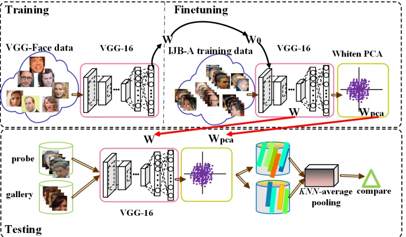
Aiming to address this Set-to-Set matching problem, in this paper, we propose a simple but effective S2S distance by leveraging the kNN-average pooling. Our recognition system starts by a deep feature extraction step making use of a VGG-16 deep network and a transfer learning technique to compensate for lack of training data. The trained model in turn is used to acquire features from all images over a set in the test phase. We employ the proposed S2S distance to calculate the similarity of two sets, and in the end make decision for the recognition tasks. The overview of the entire system is illustrated in Fig. 2 and our contributions can be summarized as the following three points:

• The primary contribution lies in a novel Set-to-Set dis-tance employingkNearest Neighbor (kNN)-average pool-ing to measure the similarity between two sets of face media. The S2S distance is simple but very effective and robust to the outliers.

• Our framework built on the S2S distance is so flexible that

different metrics including both pre-defined and learned ones can be incorporated. The experimental results reveal that there is no need to learn a particular metric for such a challenging dataset wherein many subjects are with very limited media samples, even sometimes with only one sample.

• Compared with feature-pooling, score-pooling and even some deep learning methods, our simple S2S distance helps to achieve the state-of-the-art results on IJB-A which is the only set-based face dataset.

The rest of the paper is organized as follows. In Section II we review the latest works on the IJB-A dataset and make a brief discussion. Afterwards, our motivation and method are presented in Section III. Section IV details the experiments to demonstrate the effectiveness and flexibility of our approach followed by a conclusion and our future work in the last section.

II. RELATEDWORK

As described in the previous section, earlier recognition methods obtained quite low accuracies under the unconstrained settings. In order to improve the recognition performance on the datasets over images, some researchers dedicated to finding better face representations or descriptors. In [14], the authors used Fisher vectors on densely sampled SIFT and then compressed the encoding to a small representation. Apart from the descriptor-based methods, feature selection/compression and metric learning [15], [16], [17] also made some contri-butions to improve the face recognition under unconstrained environments.

Furthermore, some previous methods dealing with the set-based setting,e.g., the YTF benchmark, were also developed. In this database, the probe and the gallery were typically comprised of multiple frames from the same video. The simple way was to generate one feature by computing the mean of all features in each set and then compare the two aggregated features of the two given sets. One elaborate method designed for this purpose was convex hull [18] which performed well when many frames were available in sets. Under the assumption that the elements in a set may lie close to a linear subspace, subspace-based methods [19] were introduced. To overcome the drawbacks of the traditional kernel-based methods, Huang et al. [20] proposed a method to learn the projection metric directly from a Grassmann manifold. Moreover, various distribution based representations were considered, such as the Bag of Features [21](BF) and Vector of Locally Aggregated Descriptors (VLAD) [22].

This article has been accepted for publication in a future issue of this journal, but has not been fully edited. Content may change prior to final publication. Citation information: DOI 10.1109/TCSVT.2017.2710120, IEEE Transactions on Circuits and Systems for Video Technology

IEEE TRANSACTIONS ON CIRCUITS AND SYSTEMS FOR VIDEO TECHNOLOGY 3

Fig. 2: Overview of the entire system with three phases are included. Training: VGG-16 trained on VGG-Face data; Finetuning: Finetune pre-trained model on IJB-A training data; Testing: Using fine-tuned model to extract features and applying kNN-average pooling on extracted features.

SVM classifiers [33] were generated for both gallery and probe sets. However, it does not seem to be practical to find appropriate negative and subject-disjoint positive samples for the probe set, because the subject labels of the probe set were not always available in real applications.

III. MOTIVATION ANDMETHOD

A. Motivation

As described above, in order to push the unconstrained face recognition research close to the real-world applications, the IJB-A dataset over sets of media (images and/or videos) was released. It is understandable that a set of media rather than a single image/video provided for a subject means that more information can be available for recognition, which should be helpful for achieving better results. However, it is not always like this, especially in reality due to many uncontrolled factors. On the one hand, the great variety in age, pose, expression, illumination and other conditions, makes the set heterogeneous in contents. On the other hand, incorrect results caused by preprocessing such as face detection and alignment may introduce noise to sets. Even by looking at the ground-truth boxes provided by IJB-A, one can easily notice that they are unstable and some of them are labeled incorrectly. At the same time, we find a few persons are given wrong subject labels in the dataset. In such a Set-to-Set matching problem, given a noisy but practical dataset, the key is to avoid skewing matching scores caused by the complex factors. Essentially, we should decide which media are useful for comparison and how to weigh the similarity scores of different cross-set media pairs. From this point of view, previous strategies adopting either feature pooling or score pooling cannot generalize well in many practical cases. We make an in-depth analysis

following a preliminary definition. A feature representation

z=f(x)is a mappingf(x)∈Rdfrom an image or a framex to an encodingzwith dimensionalityd. Letz˜= 1

m

P xf(x) be the average of features of images or frames in media S, such as the average encoding for allmframes in a video.

Feature-average Poolingis proposed as a useful approach for endowing the features with invariant properties. Both image-based average pooling and media-based feature-average pooling were used in [24], in which the former takes a component wise average of the features over all the images or/and frames in a set P={z1P, z2P, . . . , znP}. Hence, the final representation isFP =

1

kPk P

zz

P_{.kPkis the number}

of images or/and frames within the set. The latter firstly con-ducts an intra-media average and then combines them via an inter-media average. Hence, there areP={˜zP

1,z˜P2, . . . ,˜znP} andFP =

1

kPk P

˜

z˜z

P_{, where kPk is the number of media}

in the set. The similarity betweenPandGcan be defined as:

Fig. 3: Illustrations of the three pooling methods. (a) feature-average pooling; (b) score-feature-average pooing; (c) kNN-average pooling (k = 1). In the probe set, the faces marked by red triangle can be seen as bad examples. In (c), the green line is from each sample in the probe set to its corresponding NNin gallery set; the orange line is from each sample gallery set to its corresponding NN in the probe set.

is likely to be close to an extreme pose. For both cases, the similarity score may not be high if any of two average features is adopted. Thus, the feature-average pooling may cause the loss of key information.

Score-average Poolingmeans the final feature is generated by averaging the calculated pairwise similarity scores (based on media features) of two sets. Given a probe set P =

{z˜P

1,z˜2P, . . . ,z˜nP} and a gallery set G = {z˜1G,z˜2G, . . . ,z˜lG}, the similarity score is represented as:

simscore aver=

1

kPk ·

1

kGk X

i,j

K(˜z_iP,z˜G_j), (2)

Obviously, the operation is fragile to outliers because it assigns equal weights even for outliers, which will definitely affect the final decision. Moreover, score-max pooling is tried in [25] but it is not robust to noises either.

B. kNN-average pooling

In view of the above analysis, we can draw a conclusion that either of feature-average pooling and score-average pooling may not properly handle the case when two sets have variable contents and noises. Aiming to solve this problem, we propose a simple but effective method called kNN-average pooling.

TABLE I: Pairwise Cosine Similarity Scores Between Probe Set and Gallery Set. The red boxes label the low scores from extreme poses and noises. Finally, our kNN-average pooling uses the scores in the green circles

kNN-average Pooling basically takes advantage of two kinds of pooling of the pairwise similarity scores between a probe set P = {z˜P

1,˜z2P, . . . ,z˜nP} and a gallery set G = {z˜G

1,z˜G2, . . . ,z˜Gl }. For each media item ˜z P

i in the probe set, we first calculate the similarity betweenz˜P

i and its knearest neighborsz˜G

N Nk in the gallery set and sum them:

sim_˜zP i =

k X

j=1

K(˜zP_i ,z˜G_{N Nj}), (3) and then take the average of all the scores as the similarity from the probe to the gallery

simP−GN N =

1

kPk P

isimz˜P i ,

Likewise, we do the same for the gallery set to get the similarity from the gallery to the probe

sim_z˜G j =

Pk i=1K(˜z

P N Ni,˜z

G j),

simG−PN N =

1

kGk P

jsimz˜G j .

Finally, the similarity between the two sets is

This article has been accepted for publication in a future issue of this journal, but has not been fully edited. Content may change prior to final publication. Citation information: DOI 10.1109/TCSVT.2017.2710120, IEEE Transactions on Circuits and Systems for Video Technology

IEEE TRANSACTIONS ON CIRCUITS AND SYSTEMS FOR VIDEO TECHNOLOGY 5

(a) (b)

Fig. 4: t-SNE visualization of deep features of 10 classes randomly selected from test dataset of split 1 after whiten PCA (a) and PCA (b).

deep features (from a VGG-face model fine-tuned on IJB-A training data) and Cosine similarity metric to calculate the three similarity measurements. Here, we set k= 1. From the figure, both feature-average pooling and score-average pooling obtain lower similarity scores for the two sets from the same subject. On the contrary, kNN-average pooling gets a higher matching score. Intuitively,kNN-average pooling behaves like a weighting strategy to select more good-samples and less bad-samples. We also list the pairwise scores based on Cosine metric in TABLE I. It can be observed that the faces with the extreme poses and the noisy images always generate low scores. Next, we present our idea from a naive probabilistic formulation perspective.

C. Naive probabilistic formulation

As we mentioned above, face recognition can be regarded as a classification problem, which checks whether the probe is the same subject class with a reference or which subject class in the gallery the probe belongs to. Given a new probe image set P, we need to find its subject class G. Based on probability theory, the maximum-a-posteriori (MAP) classifier minimizes the average classification error [34], [35]:

ˆ

G= arg maxGp(G|P).

Usually, Maximum-Likelihood (ML) is used to represent MAP when the class prior p(G)is uniform:

ˆ

G= arg maxGp(G|P) = arg maxGp(P|G).

If a probe setPcontains some elementsz˜1P,z˜2P, . . . ,z˜nP, under the Naive-Bayes assumption, the probability of P belonging toGis modeled as:

p(P|G) =p(˜zP

1,z˜2P, . . . ,z˜nP|G) = Q

ip(˜z P i |G). Combine the two formulas and take the log format,

ˆ

G= arg max

G log(p(G|P)) = arg maxG

n X

i

logp(˜zP_i |G) (5) According to Eq. 5, we need to calculate the probability den-sityp(˜zP|G)of elements ˜zPin galleryG. Referring to [34], we get an estimationpˆ(˜zP|G)as:

ˆ

p(˜zP|G) = 1

l

l X

j=1

K(˜zP,z˜_jG) (6)

Furthermore, an accurate approximation of Eq. 6 using (few)

klargest elements in the sum is given below:

pN N(˜zP|G) =

1

l

k X

j=1

K(˜zP,˜z_{N N}G

j) (7) Theseklargest elements correspond to theknearest neighbors of an elementz˜P _{∈P within the elementsz˜}G

1,z˜G2, . . . ,z˜lG ∈ G. This is the probability model of ourkNN-average pooling method. Due to thatlis a constant, we approximate a similarity defined in Eq. 3. To match two sets, we apply a symmetric format in Eq. 4.

D. Pre-defined metrics embedded vs Learned metrics embed-ded

(a) (b)

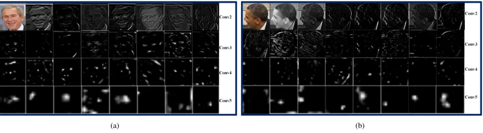
Fig. 5: Visualization of deep features from Conv2, Conv3, Conv4 and Conv5. (a) Frontal face; (b) Profile face. Most of the reaction hits on eyes, noses, mouths and ears which are most important for face recognition.

kNN-average pooling is very generic and flexible, which allows switching between several metrics (both pre-defined and learned).

Generally, supervised metric learning considers a classifi-cation problem, whose objective is minimizing the distance between intra-class samples and maximizing the distance between inter-class samples. However, there are many subjects with only one sample in the IJB-A dataset. In this case, metric learning does not seem to present a satisfactory performance due to lack of training data. Fortunately, our S2S distance embedded with the unsupervised metric can achieve fabulous results. In this paper, we endow the kernel function K(x, y)

three different metrics including Euclidean distance [36], Co-sine similarity [37] and Joint Bayesian [38], [39]. Euclidean distance and Cosine similarity are unsupervised metrics. The formulas respectively are:

dEu(˜zPi ,z˜ G j ) =kz˜

P i −˜z

G

jk2, (8)

dCos(˜ziP,z˜ G

j) = cos(˜z P i ,z˜

G j ) =

˜

zP i ·z˜jG kz˜P

i kkz˜ G j k

(9)

Moreover, the Joint Bayesian metric was introduced in previous works [39], where the appearance of a face can be modeled by two parts: identity and intra-personal variation. We use LDA to approximately optimize the loss function for JBmetric.

IV. EXPERIMENTALRESULTS

In this section, we present details of the whole system and evaluate it on the IJB-A dataset. We plot the bar figures to show the specific results for different settings. The Receiver Operating Characteristic (ROC) curves for 1:1 face verifi-cation, the Cumulative Match Characteristic (CMC) curves for 1:N closed-set face identification and the Decision Error Tradeoff (DET) curves for 1:N open-set identification are used to show all the comparisons. Our S2S distance based on kNN-average pooling really helps to improve the results significantly. Moreover, compared to the existing methods, our system achieves the state-of-the-art results.

A. Implementation details

Deep features prove to be powerful in face recognition [1], [2], [3], [40], [41], [42], [43]. Due to the fact that each split of IJB-A does not contain many images, we use transfer learning to get deep representations. Specifically, we apply 16 [44] deep network trained from scratch on the VGG-Face dataset [1] without overlapping with the IJB-A dataset and then fine-tune it on training dataset of each split of IJB-A. We crop the faces using the ground-truth boxes provided with IJB-A and then re-scale them to 224×224×3. Face alignment is not done here because not all images are provided with three key points. Another reason is that it is difficult to align different profile faces and the incorrect alignment results will bring extra noises. We input the face patches of the training set into our VGG-16 network and set the base learning rate 0.001 and learning rate policy “step”. We take the penultimate layer output as the feature encoding of 4096 dimensions. Afterwards, whitened PCA [45] is used to reduce the dimension to 256. We randomly select 10 classes from the test dataset of split 1 and use t-SNE [46] to visualize its distributions after a PCA and a whitened PCA respectively (see in Fig. 4). It is clear that whitened PCA makes the intra-class distribution like a spherical shape and increases the cohesion within the same class. The final features used forkNN-average pooling are based on media sample. In our experiments,k= 2

is used for all settings. If a set only has one media, we adjust

k= 1.

B. IJB-A evaluation

IJB-A is the only public dataset over sets, which contains in total 5,712 images and 2,085 videos of 500 subjects, with an average of 11.4 images and 4.2 videos per subject [7]. They are randomly divided into 10 splits with overlap at the subject level. There are 333 subjects randomly sampled and placed in training for each split, the other 167 subjects placed in testing. There are three protocols defined on it, which are for verification, closed-set identification and open-set identification respectively. All the results reported below are averages over the 10 splits.

This article has been accepted for publication in a future issue of this journal, but has not been fully edited. Content may change prior to final publication. Citation information: DOI 10.1109/TCSVT.2017.2710120, IEEE Transactions on Circuits and Systems for Video Technology

IEEE TRANSACTIONS ON CIRCUITS AND SYSTEMS FOR VIDEO TECHNOLOGY 7

(a) (b) (c) (d)

Fig. 6: IJB-A 1:1 ROC curve based on different metrics:(a) Cosine Similarity; (b) Euclidean Distance; (c) JB metric; (d) Comparisons between the results of kNN-average method based on the three metrics.

(a) (b) (c) (d)

Fig. 7: IJB-A 1:N CMC curve based on different metrics:(a) Cosine Similarity; (b) Euclidean Distance; (c) JB metric; (d) Comparisons between the results of kNN-average method based on the three metrics.

(a) (b) (c) (d)

Fig. 8: IJB-A 1:N DET curve based on different metrics:(a) Cosine Similarity; (b) Euclidean Distance; (c) JB metric; (d) Comparisons between the results of kNN-average method based on the three metrics.

(a) (b) (c)

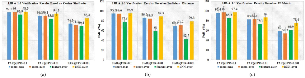
Fig. 9: IJB-A 1:1 Verification Results based on different metrics: (a) Cosine Similarity; (b) Euclidean Distance; (c)JBMetric.

of genuine pairs equals the number of probe sets, and a single gallery set is attached to each subject. The ROC curve is classically used to measure the verification accuracy.

(a) (b) (c)

Fig. 10: IJB-A 1:N Closed-set Identification Results based on different metrics: (a) Cosine Similarity; (b) Euclidean Distance; (c)JBMetric.

(a) (b) (c)

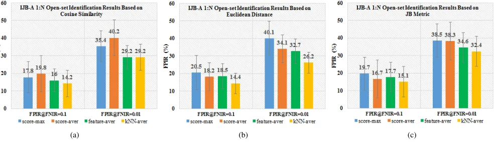
Fig. 11: IJB-A 1:N Open-set Identification Results based on different metrics: (a) Cosine Similarity; (b) Euclidean Distance; (c)JBMetric.

the false accept rate (FAR), which is the fraction of impostor pairs incorrectly exceeding the threshold. Using ROC curves, the following accuracies are reported: the TAR @ FAR = 0.1, 0.01 and 0.001. The higher the values are, the better the performance is.

We compare four pooling methods including score-max [25], score-average [26], [28], feature-average [11], [12], [13] andkNN-average pooling based on three different metrics. ROC curves are drawn for each setting in Fig. 6. Seen from the curves, ourkNN-average pooling is clearly superior, compared to the other three pooling methods, regardless of which metric is used. It is interesting to observe that the unsupervised metric Cosine similarity is even better than the supervised JB metric. The results may reveal two important points: 1) The features learned from deep Convolutional Neural Network indeed generate good representations for most faces, except for the faces with severe noise. We show the via feature maps from Conv2, Conv3, Conv4 and Conv5 layers of one frontal face and one profile face in Fig. 5. The networks have high reaction on eyes, noses, mouths and ears which are most important for face recognition. 2) Supervised JB metric does not seem to work well for the case where certain subjects only include one media, because there will be not enough samples from the same class to learn the appropriate metric parameters. In contrast, the pre-defined metrics like Cosine similarity, have

no such a limitation. That’s why Cosine similarity can get better results than the metric learning in this particular case. We also draw bar figures to show specific results of face verification (see in Fig. 9(a)-(c)). As observed from the bar figures, feature-average pooling causes the worst performance for most of the indexes. For the sets including many faces with big variation, this aggregation may lead to the leak of key information. Score-average and score-max obtain very similar results, however, both of which are sensitive to outliers. kNN-average pooling obviously outperforms them due to that it can effectively decrease the effect of noise faces. Especially for TAR@FAR=0.001, kNN-average has more than 10% im-provement compared with the others. For face verification, Cosine similarity gives the best results using kNN-average pooling. For TAR @ FAR = 0.1 and TAR @ FAR = 0.01, the top accuracies are 98.5% and 94.5%, respectively. JB metric dose not learn a good measurement due to the fact that many subjects have only one sample in the IJB-A dataset. It actually behaves similarly with Euclidean distance in terms of the performance. Overall, ourkNN-average pooling improves the results significantly.

This article has been accepted for publication in a future issue of this journal, but has not been fully edited. Content may change prior to final publication. Citation information: DOI 10.1109/TCSVT.2017.2710120, IEEE Transactions on Circuits and Systems for Video Technology

IEEE TRANSACTIONS ON CIRCUITS AND SYSTEMS FOR VIDEO TECHNOLOGY 9

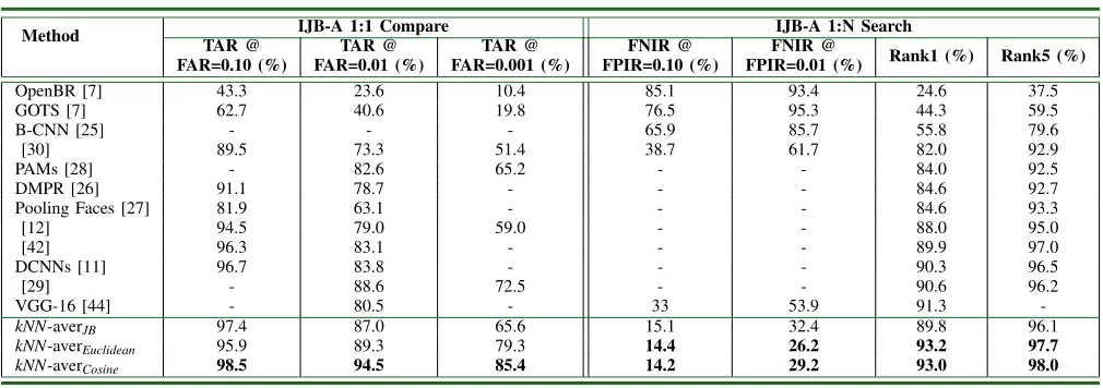
TABLE II: Performance Comparison of Different Methods

Method IJB-A 1:1 Compare IJB-A 1:N Search TAR @

FAR=0.10 (%)

TAR @ FAR=0.01 (%)

TAR @ FAR=0.001 (%)

FNIR @ FPIR=0.10 (%)

FNIR @

FPIR=0.01 (%) Rank1 (%) Rank5 (%)

OpenBR [7] 43.3 23.6 10.4 85.1 93.4 24.6 37.5

GOTS [7] 62.7 40.6 19.8 76.5 95.3 44.3 59.5

B-CNN [25] - - - 65.9 85.7 55.8 79.6

[30] 89.5 73.3 51.4 38.7 61.7 82.0 92.9

PAMs [28] - 82.6 65.2 - - 84.0 92.5

DMPR [26] 91.1 78.7 - - - 84.6 92.7

Pooling Faces [27] 81.9 63.1 - - - 84.6 93.3

[12] 94.5 79.0 59.0 - - 88.0 95.0

[42] 96.3 83.1 - - - 89.9 97.0

DCNNs [11] 96.7 83.8 - - - 90.3 96.5

[29] - 88.6 72.5 - - 90.6 96.2

VGG-16 [44] - 80.5 - 33 53.9 91.3

-kNN-averJB 97.4 87.0 65.6 15.1 32.4 89.8 96.1

kNN-averEuclidean 95.9 89.3 79.3 14.4 26.2 93.2 97.7

kNN-averCosine 98.5 94.5 85.4 14.2 29.2 93.0 98.0

set. But each probe set is to be searched against the gallery sets. Generally, closed-set is for user driven searches (e.g., forensic identification). The cumulative match characteristic (CMC) is an information retrieval metric that captures the recall of a specific probe identity within top-k most similar candidates in gallery. We report rank-1 and rank-5 correct retrieval rates (CRR) for the closed setting. However, for other applications like de-duplication, some searches cannot manually be examined. There exists a tradeoff between false alarms and misses. In this case, the decision error tradeoff (DET) is plotted to measure the false positive identification rate (FPIR) and false negative identification rate (FNIR). FPIR means the false alarm rate which measures what fraction of comparisons between probe sets and non-match gallery set result in a similarity score above a given thresholdt. FNIR is the miss rate measuring what fraction of probe searches fail to match a mated gallery set above t. In this paper, FPIR @ FNIR = 0.1 and 0.01 will be reported. The lower the values are, the better the performance is.

For 1: N closed-set face identification, we also compare the four pooling methods using Cosine similarity, Euclidean distance and JB. The CMC curves for all the settings can be found in Fig. 7. The kNN-average pooling presents a signif-icant increment especially for rank-1 of the three embedded metrics. In Fig. 7(d), the comparisons for the three metrics based on kNN-average pooling are shown, in which both Cosine embedded and Euclidean embedded perform similarly but are much better than JBembedded. Fig. 10(a)-(c) display the numeric results for closed-set. Generally, the results of score-max and score-average are more or less the same. Using Cosine similarity, kNN-average pooling achieves a top accuracy of 98% for rank-5 and gets the best result of 93.2% for rank-1 if applying Euclidean distance.JBembedded gives 92.1% and 97.4% respectively for rank-1 and rank-5 based on kNN-average pooling, which help to increase the correct retrieval rate among different pooling methods.

The more challenging task is 1: N open-set identification, which requires rejecting the subjects without the enrollment in gallery. Fig. 11(a)-(c) list the results based on the four pooling

methods respectively using Cosine similarity embedded, Eu-clidean distance embedded and JB embedded. It is interesting to find that feature-average pooling performs better than the other two score-related pooling methods at FNIR@FPIR=0.01. It seems that feature-average representation for the subjects not enrolled in gallery can get a low score, which may help to de-crease the miss rate. However,kNN-average pooling still is the best strategy for open-set. It decreases the miss rate by 1.8% for FNIR@FPIR=0.1 when Cosine similarity is embedded. Furthermore, for FNIR@FPIR=0.1 and FNIR@FPIR=0.01, there are more than 4% and 6% misses decreased, compared with the other three pooling methods using Euclidean distance. In Fig. 8, 1: N DET curves show the visual results. The results of feature-average pooling are close to those of score-average pooling but still worse than thekNN-average pooling. It reaches the same conclusion that unsupervised metrics can outperform supervised metric learning, which further supports our simple but efficient S2S distance.

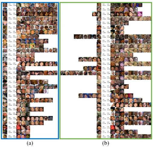
Fig. 12: Failure cases analysis. (a) Top 30 worst matched; (b) Top 30 worst Non-matched. Most face sets just contain one media and most faces are very profile.

by the very limited number of media in a set. In future, we hope to utilize synthesized images to augment data for subjects with limited samples. We assume enough samples of a subject should address the problem.

4) Comparisons with benchmarks: We compare our meth-ods using different metrics with the existing 12 methmeth-ods from other publications. OpenBR and GOTS are two basic baselines given in [7]. They are not deep learning methods and give very poor performances for both verification and identification. Other methods using deep convolutional networks, which were introduced in Section II, have some improvements. Not all of the methods performs on all protocols of IJB-A. For example, B-CNN method just focuses on face identification and gets the accuracy of 55.8% for rank-1, and the missed rate of 85.7% for FPIR=0.01. Most of the other methods only concentrated on the face verification task and closed-set identification. DCNNs [11] shows the best results among these benchmarks in TABLE II. However, we test all the pro-tocols of IJB-A using kNN-average pooling based on Cosine similarity, Euclidean distance and JB metric. The results of the three settings are very competitive. Especially, the two unsupervised metrics embedded get top accuracies over most of all protocols. EvenJBembedded achieve 15.1% and 32.4% respectively for FNIR@FPIR=0.1 and 0.01, which are much better than the previous results. Seen from the table, kNN-average pooling using Cosine similarity further exceeds other methods for face verification and closed-set face identification and kNN-average pooling using Euclidean distance generates large margins over other methods. In all, even though the kNN-average pooling combing with unsupervised metrics is simple, it is very effective and flexible.

V. CONCLUSION

In this paper, we have presented a very simple but effective S2S distance to measure the similarity between two image sets, which is suitable for addressing the identification of faces with heterogeneous contents, such as the IJB-A dataset. The S2S distance is defined based on averaging a mutual comparison between the probe set and the gallery set, in which each element is only compared with its nearest neighbors. By doing so, the impact of outliers and noises commonly occurring in the IJB-A dataset is under control. Furthermore, variable metric methods can be embedded into the proposed S2S distance measure. Finally, we showed that even with a simple unsupervised metric, like Euclidean distance, the proposed method can achieve competitive accuracy for both face verification and identification. Furthermore, the kNN-average pooling is very generic and can be potentially applied to various applications over sets, where some severe noise or extreme cases occur caused by capturing conditions in real world. Such applications include person-reidentification [47], object recognition, saliency detection [48], [49] and image retrieval [50].

In future work, our system can be enhanced from two aspects: (1) we will embed thekNN-average pooling to a deep network in an end-to-end fashion. We believe such a strategy will further boost the recognition performance; (2) We will investigate the local features based on extracting key points from faces and design a S2S distance based on these local features, enabling more robust matching between faces with severe variations.

REFERENCES

[1] O. Parkhi, A. Vedaldi, and A. Zisserman, “Deep face recognition,” in British Machine Vision Conference, 2015.

[2] Y. Taigman, M. Yang, M. A. Ranzato, and L. Wolf, “Deepface: Closing the gap to human-level performance in face verification,” in IEEE Conference on Computer Vision and Pattern Recognition, 2014. [3] F. Schroff, D. Kalenichenko, and J. Pjilbin, “Facenet: A unified

em-bedding for face recognition and clustering,” in IEEE Conference on Computer Vision and Pattern Recognition, 2015.

[4] Y. Taigman, M. Yang, M. A. Ranzato, and L. Wolf, “Web-scale training for face identification,” in IEEE Conference on Computer Vision and Pattern Recognition, 2015.

[5] G. Huang, M. Ramesh, T. Berg, and E. Learned-Miller, “Labeled faces in the wild: A database for studying face recognition in unconstrained environments,” University of Massachusetts, Tech. Rep. TR-07-49, 2007. [6] N. Kumar, A. C. Berg, P. N. Belhumeur, and S. K. Nayar, “Attribute and simile classifiers for face verification,” inInternational Conference on Computer Vision, 2009.

[7] B. Klare, B. Klein, E. Taborsky, A. Blanton, J. Cheney, K. Allen, P. Grother, A. Mah, and A. Jain, “Pushing the frontiers of unconstrained face detection and recognition: Iarpa janus benchmark a,” in IEEE Conference on Computer Vision and Pattern Recognition, 2015. [8] L. Wolf, T. Hassner, and I. Maoz, “Face recognition in unconstrained

videos with matched background similarity,” in IEEE Conference on Computer Vision and Pattern Recognition, 2011.

[9] J. Han, D. Zhang, X. Hu, L. Guo, J. Ren, and F. Wu, “Background prior-based salient object detection via deep reconstruction residual,” IEEETrans.Circuits and Systems for Video Technology, vol. 25, no. 8, pp. 1309–1321, 2015.

[10] J. Zabalzaa, J. Rena, J. Zhengb, H. Zhaoc, C. Qingd, Z. Yange, P. Duf, and S. Marshalla, “Novel segmented stacked autoencoder for effective dimensionality reduction and feature extraction in hyperspectral imaging,”Neurocomputing, vol. 185, pp. 1–10, 2016.

This article has been accepted for publication in a future issue of this journal, but has not been fully edited. Content may change prior to final publication. Citation information: DOI 10.1109/TCSVT.2017.2710120, IEEE Transactions on Circuits and Systems for Video Technology

IEEE TRANSACTIONS ON CIRCUITS AND SYSTEMS FOR VIDEO TECHNOLOGY 11

[12] S. Sankaranarayanan, A. Alavi, and R. Chellappa, “Triplet similarity embedding for face verification,” 2016.

[13] S. Sankaranarayanan, A. Alavi, C. Castillo, and R. Chellappa, “Triplet probabilistic embedding for face verification and clustering,” 2016. [14] K. Simonyan, O. M. Parkhi, A. Vedaldi, and A. Zisserman, “Fisher

vector faces in the wild,” inBritish Machine Vision Conference, 2013. [15] D. Tao, Y. Guo, M. Song, Y. Li, Z. Yu, and Y. Tang, “Person

re-identification by dual-regularized kiss metric learning,” IEEETrans. Image Processing, vol. 25, no. 6, pp. 2726–2738, 2016.

[16] D. Tao, J. Cheng, X. Gao, and C. Deng, “Robust sparse coding for mobile image labeling on the cloud,”IEEETrans.Circuits and Systems for Video Technology, vol. 27, no. 1, pp. 62–72, 2017.

[17] D. Tao, L. Jin, Y. Wang, Y. Yuan, and X. Li, “Person re-identification by regularized smoothing kiss metric learning,”IEEETrans.Circuits and Systems for Video Technology, vol. 23, no. 10, pp. 1675–1685, 2013. [18] H. Cevikalp and B. Triggs, “Face recognition based on image set,” in

IEEE Conference on Computer Vision and Pattern Recognition, 2010. [19] J. Hamm and D. D. Lee, “Grassmann discriminant analysis: A

unify-ing view on subspace-based learnunify-ing,” inInternational Conference on Machine Learning, 2008.

[20] Z. Huang, R. Wang, S. Shan, and X. Chen, “Projection metric learning on grassmann manifold with application to video based face recogni-tion,” inIEEE Conference on Computer Vision and Pattern Recognition, 2015.

[21] S. Labeznik, C. Schmid, and J. Ponce, “Beyond bags of features: Spatial pyramid matching for recognizing natural scene categories,” inIEEE Conference on Computer Vision and Pattern Recognition, 2006. [22] H. Jegou, M. Douze, C. Schmid, and P. Perez, “Aggregating local

descriptors into a compact image representation,” inIEEE Conference on Computer Vision and Pattern Recognition, 2010.

[23] D. Yi, Z. Lei, S. Liao, and S. Z. Li, “Learning face representation from scratch,” 2014.

[24] A. Krizhevsky, I. Sutskever, and G. E. Hinton, “Image classification with deep convolutional neural networks,” inin Advances in neural information processing system, 2012, pp. 1097–1155.

[25] A. RoyChowdhury, T.-Y. Lin, S. Maji, and E. Learned-Miller, “One-many face recognition with bilinear cnns,” inIEEE WACV, 2016. [26] W. AbdAlmageed, Y. Wu, S. Rawls, S. Harel, T. Hassner, I. Masi,

J. Choi, J. Lekust, J. Kim, P. Natarajan, R. Nevatia, and G. Medioni, “Face recognition using deep multi-pose representation,” inIEEE WACV, 2016.

[27] T. Hassner, I. Masi, J. Kim, J. Choi, and S. Harel, “Pooling faces: Template based face recognition with pooled face images,” in IEEE Conference on Computer Vision and Pattern Recognition, 2016. [28] I. Masi, S. Rawls, G. Medioni, and P. Natarajan, “Pose-aware face

recognition in the wild,” inIEEE Conference on Computer Vision and Pattern Recognition, 2016.

[29] I. Masi, A. T. Tran, J. T. Leksut, T. Hassner, and G. Medioni, “Do we really need to collect millions of faces for effective face recognition?” inEuropean Conference on Computer Vision, 2016.

[30] D. Wang, C. Otto, and A. K. Jain, “Face search at scale: 80 million gallery,” MSU, Tech. Rep. MSU-CSE-15-11, 2015.

[31] R. Chellappa, J.-C. Chen, R. Ranjan, S. Sankaranarayanan, A. Kumar, V. M. Patel, and C. D. Castillo, “Towards the design of an end-to-end automated system for image and video-based recognition,” http: //ita.ucsd.edu/workshop/16/files/paper/paper 2663.pdf.

[32] N. Crosswhite, J. Byrne, O. M. Parkhi, C. Stauffer, Q. Cao, and A. Zis-serman, “Template adaptation for face verification and identification,” 2016.

[33] J. Ren, “Ann vs. svm: Which one performs better in classification of mccs in mammogram imaging,”Knowledge-Based Systems, vol. 26, pp. 144–153, 2012.

[34] O. Boiman, E. Shechtman, and M. Irani, “In defense of nearest-neighbor based image classification,” inIEEE Conference on Computer Vision and Pattern Recognition, 2008.

[35] R. Duda, P. Hart, and D. stork,Patten classification. Wiley, New York, 2001.

[36] K. Weinberger, J. Blitzer, and L. Saul, “Distance metric learning for large margin nearest neighbour classification,” inin Advances in neural information processing system, 2006, pp. 1473–1480.

[37] H. V. Nguyen and L. Bai, “Cosine similarity metric learning for face verification,” inAsian Conference on Computer Vision, 2010. [38] D. Chen, X. Cao, L. Wang, F. Wen, and J. Sun, “Bayesian face revisited:

A joint formulation,” inEuropean Conference on Computer Vision, 2012. [39] B. Moghaddam, T. Jebara, and A. Pentland, “Bayesian face recognition,”

Pattern Recognition, pp. 1771–1782, 2000.

[40] Y. Sun, D. Liang, X. Wang, and X. Tang, “Deepid3: Face recognition with very deep neural networks,” 2015.

[41] Y. Sun, X. Wang, and X. Tang, “Deeply learned face representations are sparse, selective, and robust,” inIEEE Conference on Computer Vision and Pattern Recognition, 2015.

[42] J. Hu, J. Lu, and Y. P. Tan, “Discriminative deep metric learning for face verification in the wild,” inIEEE Conference on Computer Vision and Pattern Recognition, 2014.

[43] E. Zhou, Z. Cao, and Q. Yin, “Naive-deep face recognition: Touching the limit of lfw benchmark or not?” 2015.

[44] K. Simonyan and A. Zisserman, “Very deep convolutional networks for large-scale image recognition,” 2014.

[45] H. V. Nguyen, L. Bai, and L. Shen, “Local gabor binary pattern whitened pca: A novel approach for face recognition from single image per person,” inn Advances in Biometrics, 2009, pp. 269–278.

[46] L. Maaten and G. Hinton, “Visualizing data using t-sne,” Journal of Machine Learning Research, 2008.

[47] S. Tan, F. Zheng, L. Liu, J. Han and L. Shao, “Dense Invariant Feature Based Support Vector Ranking for Cross-Camera Person Re-identification,”IEEE Trans.Circuits and Systems for Video Technology, DOI: 10.1109/TCSVT.2016.2555739, 2017.

[48] D. Zhang, J. Han, J. Han and L. Shao, “Cosaliency Detection Based on Intrasaliency Prior Transfer and Deep Intersaliency Mining,”IEEETrans. Nerual Networks and Learning Systems, vol. 27, no. 6, pp. 1163–1176, 2016.

[49] D. Zhang, D. Meng, and J. Han, “Co-Saliency Detection via a Self-Paced Multiple-Instance Learning Framework.,”IEEETrans. Pattern Analysis and Machine Intelligence, vol. 39, no. 5, pp. 865–878, 2017. [50] Y. Guo, G. Ding, L. Liu, J. Han and L. Shao, “Learning to Hash

With Optimized Anchor Embedding for Scalable Retrieval,”IEEETrans. Image Processing, vol. 26, no. 3, pp. 1344–1354, 2017.

Jiaojiao Zhaocurrently is a Ph. D. candidate with the Department of Computer Science at Northumbria University, UK.

Jungong Hanis a faculty member with the School of Computing and Communications at Lancaster University, Lancaster, UK. Previously, he was a senior lecturer with the Department of Computer and Information Sciences at Northumbria University, UK.