warwick.ac.uk/lib-publications
Manuscript version: Author’s Accepted Manuscript
The version presented in WRAP is the author’s accepted manuscript and may differ from the
published version or Version of Record.
Persistent WRAP URL:
http://wrap.warwick.ac.uk/110758
How to cite:
Please refer to published version for the most recent bibliographic citation information.
If a published version is known of, the repository item page linked to above, will contain
details on accessing it.
Copyright and reuse:
The Warwick Research Archive Portal (WRAP) makes this work by researchers of the
University of Warwick available open access under the following conditions.
Copyright © and all moral rights to the version of the paper presented here belong to the
individual author(s) and/or other copyright owners. To the extent reasonable and
practicable the material made available in WRAP has been checked for eligibility before
being made available.
Copies of full items can be used for personal research or study, educational, or not-for-profit
purposes without prior permission or charge. Provided that the authors, title and full
bibliographic details are credited, a hyperlink and/or URL is given for the original metadata
page and the content is not changed in any way.
Publisher’s statement:
Please refer to the repository item page, publisher’s statement section, for further
information.
An automated search for transiting exocomets
Grant M. Kennedy,
1
,
2
?
Greg Hope,
3
Simon T. Hodgkin,
3
Mark C. Wyatt
3
1Department of Physics, University of Warwick, Gibbet Hill Road, Coventry, CV4 7AL, UK
2Centre for Exoplanets and Habitability, University of Warwick, Gibbet Hill Road, Coventry, CV4 7AL 3Institute of Astronomy, University of Cambridge, Madingley Road, Cambridge CB3 0HA, UK
Accepted XXX. Received YYY; in original form ZZZ
ABSTRACT
This paper discusses an algorithm for detecting single transits in photometric time-series data. Specifically, we aim to identify asymmetric transits with ingress that is more rapid than egress, as expected for cometary bodies with a significant tail. The algorithm is automated, so can be applied to large samples and only a relatively small number of events need to be manually vetted. We applied this algorithm to all long cadence light curves from the Kepler mission, finding 16 candidate transits with significant asymmetry, 11 of which were found to be artefacts or symmetric transits after manual inspection. Of the 5 remaining events, four are the 0.1% depth events previously identified for KIC 3542116 and 11084727. We identify HD 182952 (KIC 8027456) as a third system showing a potential comet transit. All three stars showing these events have H-R diagram locations consistent with ∼100Myr-old open cluster stars, as might be expected given that cometary source regions deplete with age, and giving credence to the comet hypothesis. If these events are part of the same population of events as seen for KIC 8462852, the small increase in detections at 0.1% depth compared to 10% depth suggests that future work should consider whether the distribution is naturally flat, or if comets with symmetric transits in this depth range remain undiscovered. Future searches relying on asymmetry should be more successful if they focus on larger samples and young stars, rather than digging further into the noise.
Key words: comets:general – circumstellar matter – planetary systems –
stars:variables:general – infrared: planetary systems – stars:individual:HD 182952.
1 INTRODUCTION
Comets are a well known and common component of our Solar system. These bodies, like the Asteroids, are planetary building blocks and are a remnant of the processes that made the giant planets. Comets sometimes appear as naked-eye objects in the night sky when they pass through the inner Solar system; while comet nuclei are relatively small and hard to detect, their comae can be much larger and more visible, in some cases as large as the Sun. These comae tend to have very low optical depths, and are generally observed in scattered light.
The first evidence that comets may exist in close prox-imity to other stars came from spectral observations, which found transient absorption features towards the young star
β Pictoris (Ferlet et al. 1987; Kiefer et al. 2014a). Fur-ther detections have been made towards oFur-ther stars, such as HD 172555 (Kiefer et al. 2014b) andφLeo (Eiroa et al. 2016). These features change from night-to-night, have
ra-? E-mail: [email protected]
dial velocities, accelerations, and absorption depths consis-tent with apparition at a few to a few tens of stellar radii, and with models of cometary comae (Beust et al. 1990;
Kennedy 2018). This discovery prompted theoretical work
that explored the possibility of detecting transiting comets in broadband photometry, predicting the depths to be of or-der tenths of a percent (Lecavelier Des Etangs et al. 1999). To date, none of the stars showing variable spectral absorp-tion have been seen to show broadband photometric variabil-ity that might be attributed to the same or similar events.
The detection of photometric variation has instead re-lied on wide-field transit surveys, where hundreds of thou-sands or millions of stars are monitored for month to decade-long periods. In particular, the detection of deep and irregu-lar dimming events inKeplerdata for KIC 8462852 renewed interest in the possibility of transiting comets (Boyajian
et al. 2016;Wyatt et al. 2018). Of the many proposed
sce-narios — including Solar System-related clouds, intervening compact objects and interstellar material, and planetary en-gulfment (e.g.Wright & Sigurdsson 2016;Makarov & Goldin
2016; Nesluˇsan & Budaj 2017) — the comet family model
©2015 The Authors
has seen the most development, and been shown to explain both the short and long term variation for KIC 8462852
(Wyatt et al. 2018).
While this star is unique among those observed by Ke-pler in terms of the depth, shape, and duration of the dimming events, there is now evidence of shallower events that appear consistent with the predictions ofLecavelier Des
Etangs et al., and that have therefore been interpreted as
exocometary transits (Rappaport et al. 2018).
The study byRappaport et al.involved examining all photometric data from theKepler mission by eye, looking for new dimming events which had not been detected by the Planet Hunters citizen scientist project (e.g. Fischer et al. 2012) or other searches. They found three transit events around the star KIC 3542116, and a similar event around KIC 11084727. These events all have a similar shape; dis-tinctly asymmetric with a steep initial drop in flux and a longer tail. The events for KIC 3542116 could have a period of about 92 days, but would then also require the depth of the events to be highly variable, as more 0.1% events should have been detected during theKepler mission if the events were periodic. Further analysis of the light curve of KIC 3542116 revealed three much shallower events of similar shape. Based on a remarkable similarity to the predictions of
Lecavelier Des Etangs et al.(1999),Rappaport et al.argue
that the most likely causes of these events are exocomets. Of the seven events discussed inRappaport et al., only four were detected in the initial visual survey. The other three were smaller events, only visible after more detailed examination of the KIC 3542116 light curve. In particular, determining the shapes of these shallow events (and thus determining their cometary nature) required target-specific analysis for subsections of the light curve near the event of interest using Gaussian processes. Whether this type of detrending could be applied to the entireKepler dataset in an automated way is unclear.
Here, we describe the development of an automated al-gorithm to perform a similar search. The primary motivation is that automated methods are less prone to human error, are repeatable, and allow specific hypotheses to be tested in ways that would be difficult (or unreasonable) compared to by-eye methods (i.e. “can you please look through those 200,000 light curves again, but this time look for feature X that we forgot to mention last time”). Specifically, our basic assumption here is that the defining feature of a photomet-ric cometary transit is an asymmetry that is caused by the coma and tail, and a metric that quantifies this asymmetry is central to our search. Section2describes theKeplerdata used, sections3and4describe our search algorithm, its ap-plication, and briefly discusses the results. We conclude in section5.
2 OBTAINING DATA
The entireKepler dataset was downloaded from the Mikul-ski Archive for Space Telescopes (MAST). In total the data comprise four years of photometry for roughly 200,000 dis-tinct stars. Not all stars were observed for the full length of the mission, so for statistical purposes we also use 150,000 as the approximate number of equivalent stars that were observed for the full mission duration.
The flux values for the light curves come in two prod-ucts, SAP FLUX and PDCSAP FLUX (see theKeplerdata processing handbook,Smith et al. 2017, for more details). The SAP FLUX (Simple Aperture Photometry) is the de-tector flux within a fixed aperture. The data are then cleaned using theKeplerPDC (Pre-search Data Conditioning) mod-ule to produce the PDCSAP FLUX. Here we start with the conditioned light curves, as many of the steps in the cleaning process dramatically improve the quality of the data. Most importantly, the light curves are de-trended with long pe-riod variations (of order several months) removed. The light curves are reasonably flat, making detecting significant de-viations from the mean simpler. Additionally, the cleaning removes or corrects many artefacts, which may otherwise be detected as transit events. While beneficial, this clean-ing comes at the cost of a few additional artefacts that are discussed below.
The light curve files contain a SAP QUALITY value for each data point. These are used to indicate events, such as cosmic rays, which may affect the reliability of the data. To detect potential transits, all points with non-zero SAP QUALITY values were discarded to remove artefacts and reduce the chance of obtaining false-positive transit de-tections. We then relaxed this criterion, to include reaction wheel zero-crossings, when quantifying transit asymmetries. For each target we opted to process quarters of data separately, rather than joining the light curves into a single 4-year curve. This option was chosen because many stars in the dataset have at least one quarter of data missing, which would make creating and processing a joined light curve much more complicated, with little benefit.
The Kepler data contain the flux values at constant (≈30 minute) intervals, known as ‘cadences’. However, there are gaps in the data. Smaller gaps of 1-2 data points are common, and are often caused by removing short duration anomalies as described above. These short gaps were linearly interpolated. Larger gaps are hard to accurately fill without potentially introducing artefacts, so were treated differently as described below. The light curves were normalised by di-viding by the mean.
3 THE SEARCH ALGORITHM
3.1 Removing Periodic Noise
Many light curves contain periodic or quasi-periodic varia-tion. This may be caused by intrinsic stellar variability or surface features such as starspots. Since the events we are searching for are not expected to appear periodic (i.e. comet periods are typically longer than the 4-year duration of the
Kepler mission), we attempted to detect all significant pe-riodic signals and subtract them from the flux to produce a cleaned light curve.
not the case and there are some gaps in the data. Filling these gaps using interpolation would be required to make this method work, potentially losing accuracy.
Instead of Fourier methods, Lomb-Scargle methods were chosen. These fix our problems with Fourier transforms; computing a Lomb-Scargle periodogram does not require points to be evenly spaced without gaps, so interpolating across large gaps is not needed. It can also handle frequen-cies with non-integer cycles per oscillation, which means this method may also be more accurate. This paper uses the python implementation (VanderPlas & Ivezi´c 2015) of the fast O(NlogN) method developed byPress & Rybicki
(1989).
For each light curve, the Lomb-Scargle periodogram is computed. The highest peak, corresponding to the most sig-nificant frequency is then found. A sine wave with this fre-quency is fitted to the data as an approximation to the pe-riodic noise, which is then subtracted from the flux. This process is repeated until no peaks with a power >0.05 re-main in the periodogram, and the light curve is considered “cleaned”. Removing signals with lower power did not yield
significantly cleaner light curves.
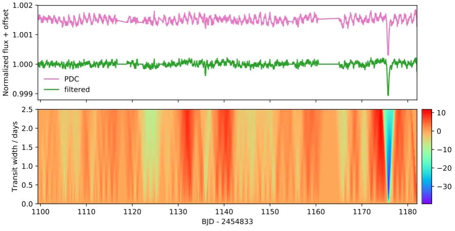
Figure 1 shows an example of this process for KIC 3542116. The variation has been reduced but the transit itself has not, improving the signal to noise of the detection. Also, the cometary shape of the transit is more visible after the processing, which will improve the model fitting.
This process takes around 1 second per light curve, and is the slowest part of the entire algorithm. The same algo-rithm using Fourier methods would be much faster (<0.1s per light curve), however it was decided the loss of accuracy would be too large.
3.2 Detecting Single Transits
To detect single transits a simple box-fit approach was used. The light curve data consists of time valuestiand normalised flux valuesxi,i=1...N. In order to keep the analysis simple, it is assumed that the time values are evenly spaced with ti−ti−1 =∆t a constant. This is true for the vast majority of the data, although, as described above, some gaps exist. These larger gaps (often of length∼1day) had the flux set to the mean value to prevent fitting of transits in missing data. Thus, while the width of a transit event may be longer than found by this search if it begins or ends with a data gap, the depth and signal to noise ratio are not affected.
In the case of Gaussian noise, the test would use a null hypothesis of white noise with
xi∼Normal(1, σx2) (1) where xi are all independent andσx is a known value that can be empirically measured for each light curve. The alter-native hypothesis for a transit of depth µ centred at time tn with width2w∆t(i.e. 2wis the number of data points a transit spans) is
xi∼
Normal(1−µ, σx2) n−w<i6n+w,
Normal(1, σx2) otherwise.
(2)
The likelihood ratio test gives a test statistic of
Tn,w=
(x¯n,w−1)
√
2w
σx
, x¯n,w =
1 2w
n+w Õ
i=n−w+1
xi (3)
where, under the null hypothesis,
Tn,w∼Normal(0,1) (4) for alln,w. A transit is indicated by a large negative value ofTn,watntr,wtr. In practise we find that the expectation of a normally distributedTn,w is not met, presumably because residual astrophysical variations in the data violate the as-sumption of Gaussian and independentxi, and we therefore use the empirical criterion described below.
This statistic can be calculated for all n = 1...N and all w up to some maximum transit width. The maximum transit width was chosen by looking at the durations of the events found inRappaport et al.(2018). The longest events found were slightly over 1 day long. We therefore use a maxi-mum transit width of approximately double that at 2.5 days. WithKepler’slong cadence of∆t≈30 minutes, this duration corresponds to wmax ≈60. The strongest event in a given light curve occurs at Ttr, the most negative value ofTn,w. Figure1showsTn,w for the filtered light curve segment in the top panel, which shows a strong detection of the transit occurring on day 1175.
The next step is to calculate the signal to noise ratio (s/n) of this transit. For this we use the distribution ofTn,w to test how much of an outlier the potential transit is, and compute the s/n asS=−min(Ttr)/σ(Tn,w), where σ(Tn,w)is the standard deviation ofTn,w over allnandw considered. For the light curve in Figure1, the distribution ofTn,wvalues is shown in Figure 2(noting that this plot is shown on a logarithmic scale, and that the tail of values below -10 is the population of points associated with the drop in flux near day 1175). The values ofTn,w are clustered around 0, with a standard deviation of4.1, so the signal to noise ratio for the transit is37.1/4.1=9, a strong detection. While we could have usedσ(Tn,wtr)(i.e. the standard deviation of the Tn,w distribution over all natwtr), we find in practise that it makes only a small difference.
3.3 Characterising Transit Shape
TheKepler data include many sources of transits that are not comets, including exoplanets and eclipsing binary stars. In order to distinguish these events from potential cometary transits, two models were fitted to each transit, and the residuals compared.
0.999
1.000
1.001
1.002
Normalized flux + offset
PDC
filtered
1100
1110
1120
1130
1140
1150
1160
1170
1180
BJD - 2454833
0.0
0.5
1.0
1.5
2.0
2.5
Transit width / days
30
[image:5.595.66.533.127.364.2]20
10
0
10
Figure 1.A segment of the raw and filtered KIC 3542116 light curves (upper panel), and the corresponding test statisticTn,w (lower
panel). After the periodic filtering the variation in the light curve has been significantly reduced, but the transit, which is not periodic, has been affected little. The minimum value isTtr=−39.4, occurring on day 1175, with an estimated transit width of 0.5 days.
30
20
10
0
10
T
10
210
310
410
5Number
Figure 2.Distibution for transit test statisticTn,wfrom the light
curve of KIC 3542116 shown in figure1. The values are centred around 0, and the detection at the minimumTtr=−37.1is a strong
outlier.
near pericentre (i.e. when its motion is not largely radial), but exocometary comae seen in calcium absorption are seen to be larger at greater stellocentric distances (where radi-ation pressure is weaker, Beust et al. 1990), which could counteract a bias towards detecting transits away from peri-centre. In any case, as discussed byLecavelier Des Etangs
et al.(1999) we have little means of distinguishing
symmet-ric cometary transits from planetary transits, so we
sim-ply acknowledge this limitation and revisit the possibility of symmetric cometary transits in light of our conclusions.
For a symmetrical transit, such as a planet or star tran-sit, a simple 3-parameter Gaussian model was used.
xsym=1−Aexp
−(t−t0) 2
2θ2
(5)
For an asymmetrical comet transit, a modification of this function is used, with an exponential tail instead of a Gaus-sian beyond the transit centert0.
xcomet=
1−Aexph−(t−t0)2 2θ2
i
t6t0,
1−Aexpt0−t
λ t>t0.
(6)
The parameters for these models were optimized using the scipy curve_fitroutine.
The fits were performed on data within a window cen-tered on the location of minimumTn,w,ntr, after subtracting a linear trend on either side of the event. A fixed number of data from the time series array on either side ofntrwere used; for a transitwtrcadences (i.e. array indices) wide, data with indices in the rangentr±5wtr were used. Where data gaps are present near the transit, the time period covered by the window defined this way is therefore greater than 10wtr∆t. When the temporal window selected this way was more than 1.5 times wider than 10wtr∆t, the data were deemed insuffi-cient to have confidence in the out-of-transit baseline and/or the event itself.
[image:5.595.50.277.440.606.2]1174
1175
1176
1177
1178
BJD - 2454833
0.9988
0.9990
0.9992
0.9994
0.9996
0.9998
1.0000
Normalized flux
[image:6.595.311.535.102.273.2]KIC 3542116
symmetric
cometary
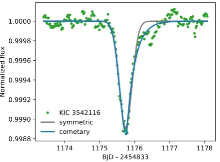
Figure 3. Symmetric and cometary models fitted to the day 1175 transit event for KIC 3542116. The comet model provides a much better fit to the data. The asymmetry value for this event isα=1.5
periodic noise removal. The linear trend was subtracted us-ing averages of the first3wtrpoints, and the lastwtrpoints, under the expectation that comet-like transits can extend farther after the transit centre than before. While this sub-traction method could in principle reduce the asymmetry of events with particularly long tails, the shape will still appear asymmetric (e.g. Figure 7suggests that the asymmetry of the event seen for KIC 11084727 could have been reduced, but this event remains the most asymmetric among those we detected).
Figure 3 shows both models fit to a single transit of KIC 3542116. A visual inspection shows the comet model to be a better fit over the symmetric model in this case. This superiority can be quantified by calculating the sum of squared residuals for each fit. We define the asymmetry parameterαto be the ratio of these two figures, that is
α=
Í(x
i−xsym(ti))2 Í(x
i−xcomet(ti))2
(7)
where the sum is taken over the 10wtr window. Values of
α >1denote a more asymmetric, comet-like transit.
The asymmetry parameter was calculated for a range of known objects. Eclipsing binary stars and exoplanets typi-cally had 0.3 . α . 1.05. The four deeper comet events found by Rappaport et al. (2018) have asymmetry values between 1.06 and 1.8. This comparison suggests that α is a good parameter to determine if a transit is likely to be a comet, with perhapsα&1.05a possible deciding character-istic.
3.4 Filtering Artefacts
The conditionedKepler data are a significant improvement over the raw time series data, but there remain artefacts that affect our ability to find asymmetric transits. Two main classes of artefacts were found which produced events with profiles looking similar to a comet transit. These would create many false positive candidates, making finding real
1010 1015 1020 1025 1030 1035 1040 1045
BJD - 2454833
0.992
0.994
0.996
0.998
1.000
1.002
1.004
1.006
1.008
Normalized flux
SAP
PDC
filtered
Figure 4.A light curve segment from the star KIC 5357069. The pink dots show the raw flux, the green dots show the processed flux (PDCSAP FLUX), and the PURPLE dots show the filtered flux. There is a sharp drop in the flux occurring on day 1027, which has not been corrected for accurately in the processing.
events difficult. This subsection discusses these classes and how they were detected and removed from the results.
The first class of artefacts occurs during a sudden in-crease or dein-crease in flux level; an example is shown in Fig-ure4. Here, the flux drops by around 1% in the duration of a single data point (less than 30 minutes), and does not rise back to initial levels. The PDC processing has attempted to fix this and flatten the curve, but has still left a large dis-continuity in the flux. In this case the disdis-continuity is then exacerbated by our filtering algorithm, because it is large. A large number of points around day 1030 lie below the av-erage, triggering a transit detection by the algorithm. The algorithm also calculates a large asymmetry for this event, with its very sharp drop in flux and a slow rise after. With-out any special handling, this event would appear to the algorithm as a likely comet.
The solution to remove this class of events is to empiri-cally look at the comet entry and exit parameters,θandλ. If one was found to be more than three times greater than the other, or if either is smaller than one tenth of a day, then one end of the light curve likely has a discontinuity and the detection is considered a false positive, so is rejected.
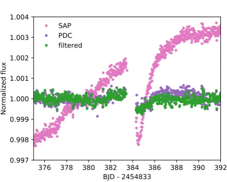
[image:6.595.50.277.107.274.2]tran-376 378 380 382 384 386 388 390 392
BJD - 2454833
0.997
0.998
0.999
1.000
1.001
1.002
1.003
1.004
Normalized flux
[image:7.595.49.274.94.274.2]SAP
PDC
filtered
Figure 5. A comet-like artefact in the data for KIC 5985654, occurring directly after a short section of missing data.
sits removed for this reason lie at 28 specific times spaced throughout theKeplermission, and therefore any real tran-sit that happened to occur at one of these times would be very hard to verify.
A similar artefact to both of the above is the so-called Sudden Pixel Sensitivity Dropout (SPSD,Smith et al. 2017), where a light curve can drop by ∼0.5% within a single ca-dence. These are generally identified and corrected by the PDC pipeline (i.e. the discontinuity is removed), but can leave artefacts that look very similar to comet transits. We did not attempt to filter these events automatically, and manually remove them from the list of candidate transiting comet systems below, either by their identification via the quality flags, or by the presence of an obvious step in the raw light curve.
4 RESULTS
The algorithm was run against the entire Kepler long-cadence dataset. Because the transit detection is indepen-dent of the shape characterization, we ran the detection al-gorithm once, and then experimented with the shape char-acterization on a subset of 67,532 transits with signal to noise ratiosSgreater than five. While we excluded all data with non-zero quality flags for transit detection, we relaxed this criterion for the shape characterization; the comet tran-sit for KIC 3542116 at day 1176 is followed by a series of reaction wheel zero-crossings, which can increase the noise level, and about 0.5 days of the egress of the day 1268 event was taken while the spacecraft was in coarse pointing. Nei-ther of these flagged periods appear to be accompanied by increased noise or systematic changes in the data. Coarse pointing data are excluded by the PDC pipeline, so we do not re-introduce those data, but we include data flagged as during zero-crossings in the shape characterization so that the day 1176 event is not excluded from our search. As seen below, this inclusion comes at the cost of some false positive detections of potential comet transits.
Of the 67,532S>5transits found with all flagged data
excluded, 36,948 potential transits remained after those con-sidered too near to gaps or light curve ends, or where model fitting failed, were excluded. Further application of the ab-solute and relative width criteria left 7,217 events. Of these, 1,336 areKepler Objects of Interest (KOIs), though most are classed as false positives and are eclipsing binaries1. By inspecting a small number of candidates, most of the events detected nearS=5are not obvious artefacts. Some appear less plausibly significant when considered in the context of the full quarter’s light curve however (e.g. in some cases showing similarly large positive excursions). It is highly un-likely that a significant fraction of these events are single transits of long-period planets; the low transit probability would imply that these belong to an implausibly numer-ous population of undetected planets, and other searches for single transits have found tens, not thousands of candidates (e.g.Wang et al. 2015).
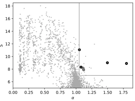
Figure6shows the signal to noise ratio and asymmetry for all 7,217 detections of the algorithm withS>5after au-tomated filtering, but before any manual filtering. The four major comet events found by Rappaport et al. (2018) are marked in black on the plot, and all lie in fairly unpopu-lated regions. However, these points also lie in what may be the tail of the distribution of more symmetric transits with
α∼1, or a population of candidate comet transits that are in fact artefacts not caught by the steps described above.
To find robust transiting comet candidates, a manual examination of the most comet-like events was therefore per-formed, informed by the region in which the events reported
byRappaport et al. (2018) lie. We therefore inspected all
candidates with signal to noise ratios greater than 7 and asymmetry parameters greater than 1.05, indicated by the grey box in figure 6. We also inspected candidates with
α >1.25 and 5 <S < 7, but found that these were either
artefacts (primarily gap-related) or cases where the fitting had failed (and that significant asymmetry was not present). Of the 16 events in the marked region, many (10) are false positives. Three are SPSD events, which can be easily identified by comparing the SAP and PDC lightcurves, and the associated quality flags. Three are increased noise dur-ing reaction wheel zero-crossdur-ings; these are also easily iden-tified by inspecting the quality flags. The behaviour in these cases appears very different to the KIC 3542116 event on day 1176, so does not appear to call the veracity of that event into question. One is a gap-related artefact. The remaining three are star or planet transits, and are for stars identified asKeplerObjects of Interest (KOIs); one is KIC 5897826, an eclipsing hierarchical triple system, where our search picked out two nearly overlapping consecutive transits of different depths on day 540 (the second was shallower, thus mas-querading as a comet-like event).
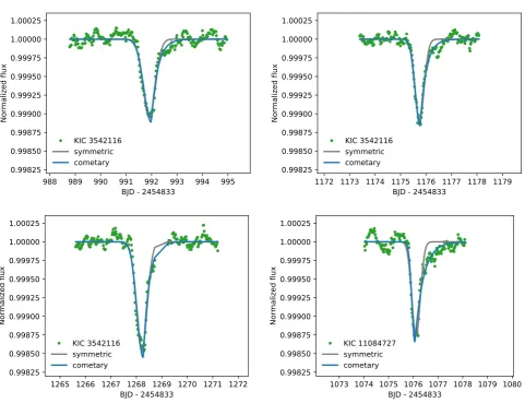
After the manual examination, 6 events were left as non-artefact events. These are shown in table 1, and four are the events identified byRappaport et al.(2018)), which are shown in Figure 7. However, whether this recovery would have been achieved for the day 1268 event for KIC 3542116 without prior knowledge of its existence is debatable. The number of events with asymmetry lower than 1.05, even at
1 Using the KOI table from the NASA Exoplanet Archive, and
0.00 0.25 0.50 0.75 1.00 1.25 1.50 1.75
6
8
10
12
14
16
18
[image:8.595.50.276.105.274.2]S
Figure 6.The signal to noise ratioS against asymmetryαfor detections, before manual filtering. The black dots correspond to the four large known events; the highest signal to noise ra-tio event to the upper left is the KIC 3542116 event on day 1268. The other events are, from left to right, KIC 3542116/d991, KIC 8027456/d1149, KIC 3129329/d901, KIC 3542116/d1175, and KIC 11084727/d1076.
relatively high s/n, is much larger than those with higher asymmetry. That is, the lower asymmetry bound for the search box in Figure6was set based on our prior knowledge of the day 1268 event, and a bound set without this knowl-edge might have been slightly higher. Figure 7 shows why the asymmetry parameter is relatively low; the spacecraft was flagged as being in coarse point for a significant part of the egress, and is thus excluded here. The data presented by
Rappaport et al. (2018) suggest that the data during this
period was not affected by pointing, and therefore that the true asymmetry for the day 1268 event is higher than 1.05. The other two events are shown in Figure 8. KIC 3129239 shows an event that is several times deeper than all others that were identified, and which visual inspec-tion shows is less asymmetric. That is, while the asymmetry parameter has a value of 1.12, this value arises in part be-cause the asymmetric model fits the data near transit center better than the symmetric model, not because the egress ap-pears more gradual than ingress. Therefore, while this event appears real (i.e. is not an artefact), it does not appear to have the characteristics of the events being searched for, and we do not consider it further. KIC 8027456 (HD 182952) shows a transit more consistent with the previously identi-fied events; the depth is about a factor of two shallower, and the width is about 50% greater. The shape is consistent with our expectation of a cometary transit, so we consider this event to be in the same class as those previously identified. The rest of the light curve for HD 182952 is unremarkable aside from two short (∼0.5d) shallow (0.25%) dips at 277 and 282 days. Both are associated with detector anomaly flags (the first during the dip, and the latter a day before-hand) and this quarter’s light curve has several step discon-tinuities of similar magnitude. We therefore do not consider these events further.
Considering HD 182952 in a little more detail, the ef-fective temperature is reported in the range 8900 to 9800K
Table 1.Comet like events in the search region which did not appear to be artefacts and were not in theKepler Objects of Interest catalogue. The date given is BJD - 2454833.
KeplerID Date SNR Asym. θ λ Depth
3542116 1268.2 11.0 1.05 0.24 0.23 0.00103 3542116 991.9 8.3 1.08 0.28 0.25 0.00074 8027456 1448.9 8.2 1.11 0.24 0.50 0.00035 3129239 900.5 7.9 1.12 0.49 0.35 0.00288 3542116 1175.7 9.0 1.50 0.19 0.24 0.00076 11084727 1076.1 8.9 1.80 0.12 0.34 0.00096
(Niemczura et al. 2015;Frasca et al. 2016), making it hotter
than both KIC 3542116 and 11084727, which are approxi-mately 6800K (Rappaport et al. 2018). By fitting stellar pho-tospheric models to the available photometry, we conclude that HD 182952 shows no evidence for an infrared excess; with only WISE observations however, the limits on poten-tial cometary source regions are poor. As was concluded for KIC 8462852, the lack of IR excess is easily consistent with the levels expected if dust is the cause of the transit event (and in any case the WISE observations occurred several years before the event, seeWyatt et al. 2018, for a discus-sion of the infra-red light curves of transiting dust). However, this conclusion relies on the assumption that stars showing such events are being viewed from a direction that places a family of comet orbits along the line of sight to the star. If the comet orbits are in fact random and could be detected by any observer (as may be implied by the different orbital properties of the deep and shallow events for KIC 3542116,
Rappaport et al. 2018), then the lack of IR excess may
pro-vide useful constraints (but such an analysis is not the goal of this paper).
The transit event for HD 182952 has a similar ingress parameter to the other events, but the egress is somewhat slower. While it seems probable that such events show a natural variation that depends on cometary activity and or-bital parameters, it may be that comets around more lumi-nous stars have longer dust tails, possibly caused by higher cometary mass loss rates.
Finally, our search does not recover the much deeper dimming events seen towards KIC 8462852, for several rea-sons. Our periodic noise removal fails badly for this star, because it assumes that any dimming events are sufficiently shallow that they do not affect the sinusoids that are fitted and subtracted. Periodic signals are therefore introduced, rather than removed, and the dimming events are affected. Also, the “D800” dimming event is well known to show the opposite asymmetry to that expected for a comet tail, and the family of “D1500” events is too complex to be reason-ably explained by single-comet models (Bodman & Quillen 2016). Otherwise, the main implication is that when consid-ering how often events of a given depth occur, we must as-sume that other searches would have found any asymmetric events that were deep enough for our search method to fail. The lack of such seems very likely to be real, as i) a search for≥5% events was performed by Boyajian et al.(2016) to look for stars similar to KIC 8462852 and none were found, and ii) any deeper comet-like events should have been dis-covered in the by-eye search described byRappaport et al.
[image:8.595.303.550.144.227.2]988 989 990 991 992 993 994 995
BJD - 2454833
0.99825
0.99850
0.99875
0.99900
0.99925
0.99950
0.99975
1.00000
1.00025
Normalized flux
KIC 3542116
symmetric
cometary
1172 1173 1174 1175 1176 1177 1178 1179
BJD - 2454833
0.99825
0.99850
0.99875
0.99900
0.99925
0.99950
0.99975
1.00000
1.00025
Normalized flux
KIC 3542116
symmetric
cometary
1265 1266 1267 1268 1269 1270 1271 1272
BJD - 2454833
0.99825
0.99850
0.99875
0.99900
0.99925
0.99950
0.99975
1.00000
1.00025
Normalized flux
KIC 3542116
symmetric
cometary
1073 1074 1075 1076 1077 1078 1079 1080
BJD - 2454833
0.99825
0.99850
0.99875
0.99900
0.99925
0.99950
0.99975
1.00000
1.00025
Normalized flux
[image:9.595.53.535.98.467.2]KIC 11084727
symmetric
cometary
Figure 7.Redetections of the events reported byRappaport et al.(2018). The data are shown within the±10wregion where the models were fit, and a linear trend has already been subtracted. All panels have the same horizontal width of 8 days, and the same vertical range.
897 898 899 900 901 902 903 904
BJD - 2454833
0.995
0.996
0.997
0.998
0.999
1.000
1.001
Normalized flux
KIC 3129239
symmetric
cometary
1445 1446 1447 1448 1449 1450 1451 1452
BJD - 2454833
0.99825
0.99850
0.99875
0.99900
0.99925
0.99950
0.99975
1.00000
1.00025
Normalized flux
KIC 8027456
symmetric
cometary
[image:9.595.53.534.533.707.2]0.0
0.2
0.4
0.6
0.8
1.0
1.2
1.4
B
PR
P1
2
3
4
5
6
7
Absolute G magnitude
0.0
0.2
0.4
0.6
0.8
1.0
1.2
1.4
B
PR
P1
2
3
4
5
6
7
[image:10.595.55.520.118.286.2]Absolute G magnitude
Figure 9.Gaia H-R diagrams for KIC 3542116, 11084727, and HD 182952 (large dots). The small dots show sets of comparison stars. The left panel uses stars within 1◦of the three of interest, and that have parallax>1, parallax s/n>50, andG<15(i.e. representative stars in theKepler field). The right panel uses stars in IC 2391, IC 2602, NGC 2451, and the Pleiades, as a set of stars approximately 100Myr old. All three stars of interest lie at the lower edge of the distribution in the left panel, and near the locus of stars in the right panel, in both cases suggesting that they are young.
4.1 Evidence for stellar youth
Figure 9 shows H-R diagrams for our three stars showing potential comet transits, compared to stars nearby on the sky (left panel) and young stars in nearby open clusters (right panel). The stars nearby on the sky were selected to be within 1◦ of any of these three stars from Gaia DR2, and restricted to have parallax >1 mas, parallax s/n> 50, and apparent G magnitude < 15 (criteria that encompass the three of interest, and are therefore representative of the stars in Kepler field). The Kepler field is near the Galac-tic plane, so this comparison allows for some spread in both the colour and magnitude of stars that is expected to arise from reddening. In the left panel our three stars of interest all fall at the lower envelope of the distribution, suggest-ing that these stars are young. The young clusters IC 2391, IC 2602, NGC 2451, and the Pleiades, were selected from
Gaia Collaboration et al. (2018) as they have similar ages
near 100Myr. In the left panel the stars with potential comet transits lie very close to the locus of these young stars, sug-gesting that their ages are not significantly greater than 100Myr.
It is well known that young nearby stars are more likely than old stars to be seen to host the bright comet reservoirs known as ‘debris disks’ (e.g. Rieke et al. 2005). Moreover, most stars that show spectral signatures of transiting comets (e.g.βPictoris, HD 172555) are also young. Thus, if the tran-siting comet hypothesis is correct for the systems identified here and byRappaport et al.(2018), then it is not surprising that these systems should also appear to be young. Indeed, the comparison in Figure9provides circumstantial evidence that this interpretation is correct.
4.2 Exocomet properties
Given that the evidence for stellar youth supports the exo-comet hypothesis, we briefly consider the properties of these putative transiting comet systems. First, we can use the
transit duration to estimate the stellocentric distance at transitrt. Rearranging equation (21) ofWyatt et al.(2018) yields
rt<27M?R?−2θ2, (8)
wherertis in units of au,M?is stellar mass inM,R?is
stel-lar radius inR andθ is the ingress parameter from Table
1in days. This equation uses2θas an estimate of the “true” transit duration, based on the expectation that the ingress is not affected by the comet tail. The inequality arises because the transit duration sets the necessary transverse velocity of the body across the face of the star, but the velocity of an eccentric orbiting body varies around the (unknown) orbit. The highest velocity occurs at the pericentre of a high eccen-tricity orbit, which sets the maximumrt, and objects with lower eccentricity or that transit away from pericentre must transit at smallerrtto have the same transverse velocity.
AssumingM?=1.5M, R?=1.5R?, andθ=0.25days
for KIC 3542116 yields an upper limit ofrt .1au, equiva-lent to a period of<300 days for a circular orbit. This limit is compatible with the possible 92-day periodicity noted by
Rappaport et al.(2018), but requires the comet activity to
be highly variable as only three events are seen during the
Kepler mission. If, on the other hand, the events are un-related, then the orbits must be eccentric with the transits occurring near pericentre in order for them to not repeat elsewhere during the Kepler mission. Assuming the same stellar properties for KIC 11084727 andθ=0.12days yields rt<0.26au, equivalent to a period of<40 days for a circular orbit. This event was not seen to repeat during theKepler
mission, again probably requiring observation of a transit near pericentre of a high eccentricity orbit, or variable ac-tivity.
For KIC 8027456, assuming M? = 2M, R? = 1.5R?,
requirement less stringent. While the orbital constraints are not strong, the duration of the events again likely requires eccentric orbits, consistent with the exocomet hypothesis.
4.3 Distribution of dimming event depths
Finally, we consider the statistics of such events. Observed phenomena commonly have a distribution of properties, and the most extreme are generally detected first. Thus, it is reasonable to expect that the dimming events seen for KIC 8462852 are the most extreme and rare of some popu-lation (Wyatt et al. 2018), which also includes the shallower events that are the focus of this paper.
In terms of the physical origin this assertion is not nec-essarily secure, as it remains uncertain whether the deep events seen for KIC 8462852 and the shallower events are the result of the same or similar phenomena, particularly given significant differences in transit characteristics. That is, while both have been interpreted as exocometary tran-sits, the evidence that led to these conclusions was different in each case. Here, we will assume that both are drawn from the same population in order to derive a depth distribution, but this population might need to have a fairly broad defi-nition, such as “circumstellar material”.
Regardless, we may consider the depth distribution of asymmetric transit events seen towards Kepler stars in purely phenomenological terms. The main caveat is that if the deep and shallow events are physically unrelated, this distribution may not be as smooth as one might expect from a single population. For example, the shallow events might in fact be the most extreme exocometary events, and KIC 8462852 has a partially or entirely different origin.
Taking the total number of stars observed as 150,0002, and assuming that all comet-like events deeper than 0.1% have been detected, the fraction of systems showing events deeper than 10% (i.e. KIC 8462852) is 1/150,000 (7×10⁻⁶). The fraction showing events deeper than 0.1% is 4/150,000 (3×10⁻⁵), though this number must be considered approxi-mate given that not all stars have the same noise properties, and that we have not carried out injection tests to verify our completeness. Comparing these numbers to Figure 14 of
Wyatt et al.(2018), the improved sensitivity (via by-eye and
automated searches) has not yielded as many new detections as suggested by that model (20 at 0.1%). The predictions for comet detections around Sun-like stars made byLecavelier
Des Etangs et al. (1999) are yet higher; equivalent to 120
detections at 0.1% for theKepler mission.
Despite the small numbers, we might conclude that the distribution of cometary transit depths is relatively flat, but this conclusion relies on all comet transits being asymmetric (and that all events are successfully identified by our algo-rithm). However, as Figure 6shows, most events are sym-metric, and given that most cannot be attributed to binary
2 Not all stars were observed in all quarters; 112,046 were
ob-served in 17 quarters, and 35,650 were obob-served in 14 quarters
(Twicken et al. 2016). Given that the transit events being
consid-ered here are rare (i.e. may only appear in one quarter’s observa-tion for a given star), we take 150,000 as an approximate number of equivalent stars that were observed for the entireKepler mis-sion
and planet transits, some may be isolated events attributable to comets, and our detection rate therefore underestimated. Our criteria for rejecting false-positives may also be too con-servative, meaning that we have missed asymmetric tran-sits, but the consistency of our results withRappaport et al.
(2018) suggests that we are not likely to have missed many at depths>0.1%.
Thus, there are various directions for future searches for comet transits. One would be to focus on distinguish-ing symmetric cometary transits from binary, planet, and other symmetric transits. Given the large number of sym-metric transits in Figure 6, this approach may be fruitful, but would need to rely on properties such as irregularity of transit timing, or transit durations that are incompati-ble with non-repetition of similar events unless the orbital eccentricity is very high. Theoretical work might also con-sider whether a flat distribution of cometary transit depths is reasonable and/or yields any insight into the comet popu-lation. The distinction between naturally symmetric transits and symmetric comet transits may be hard to make, so the obvious way to increase the number of detections, particu-larly given the small increase found here, is to increase the number of stars searched, and to focus on young stars where possible. Both K2 and TESS provide observations of stars that can help with this goal.
5 SUMMARY AND CONCLUSION
This work presents an algorithm designed to search light curves for asymmetric transits that could arise from transits of cometary bodies that orbit other stars. The asymmetry is the key discriminant here, and is based on both the expected transit shapes (Lecavelier Des Etangs et al. 1999), and those already discovered byRappaport et al.(2018). Our method first searches for single transits, and the asymmetry of these transits is then quantified. Most of the artefacts that arise due to data anomalies and post-processing are automatically rejected, but some manual inspection of a handful of light curves is required to recover ‘true’ events with confidence. For the manual search, the false positive rate was fairly low (5/16 events were classed as potential comet transits), but this success rate is very likely to be lower if the search region was expanded.
Our search recovers the three deeper transits of KIC 3542116, and the single transit of KIC 11084727, iden-tified by Rappaport et al. (2018). However, without prior knowledge of these events it is possible that one of these would have been missed because our methods finds that the level of asymmetry is relatively low due to the way we treat flagged data. We find two new events. KIC 3129239 shows a reasonably symmetric transit, whose value of the asymme-try parameter is relatively high, primarily because of a bet-ter fit near transit cenbet-ter. The level of asymmetry is there-fore not driven by slow egress, and we disregard this event. KIC 8027456 shows an event very similar to the previously known ones, albeit at a lower depth and somewhat longer duration. We consider this event as a plausible cometary transit.
have magnitudes and colours consistent with stars approx-imately 100Myr old. This signature of youth is consistent with our picture of how cometary source regions evolve; they deplete over time so the probability of witnessing comet-related events towards younger stars is presumably higher. Thus, their H-R diagram locations give credence to the comet transit hypothesis for these events.
Given the detection of∼10% deep transit events towards KIC 8462852, the detection of only a few more at 0.1% levels suggests that unless both our work and that of Rappaport
et al.(2018) has missed many events, searches for even
shal-lower asymmetric eventsmaynot yield significant numbers of new detections. While this conclusion relies somewhat on the assumption that all of these events share a similar origin, it seems that future searches are more likely to be fruitful if they focus on the possibility of symmetric cometary tran-sits, and on searching among larger and younger samples of stars.
ACKNOWLEDGEMENTS
We acknowledge valuable discussion with Tom Jacobs and Saul Rappaport. GMK is supported by the Royal Soci-ety as a Royal SociSoci-ety University Research Fellow. STH acknowledges support from an STFC Consolidated Grant. This work used the astropy Astropy Collaboration et al.
(2013), matplotlib Hunter (2007), numpy and scipy Van
Der Walt et al. (2011) python modules. An online
repos-itory with materials used in this work is available at
https://github.com/drgmk/automated exocomet hunt.
REFERENCES
Astropy Collaboration et al., 2013,A&A, 558, A33
Beust H., Vidal-Madjar A., Ferlet R., Lagrange-Henri A. M., 1990, A&A, 236, 202
Bodman E. H. L., Quillen A., 2016,ApJ, 819, L34 Boyajian T. S., et al., 2016,MNRAS, 457, 3988 Eiroa C., et al., 2016,A&A, 594, L1
Ferlet R., Vidal-Madjar A., Hobbs L. M., 1987, A&A, 185, 267 Fischer D. A., et al., 2012,MNRAS,419, 2900
Frasca A., et al., 2016,A&A,594, A39
Gaia Collaboration et al., 2018,A&A,616, A10
Hunter J. D., 2007,Computing in Science and Engineering, 9, 90 Kennedy G. M., 2018,MNRAS,
Kiefer F., Lecavelier des Etangs A., Boissier J., Vidal-Madjar A., Beust H., Lagrange A.-M., H´ebrard G., Ferlet R., 2014a, Na-ture, 514, 462
Kiefer F., Lecavelier des Etangs A., Augereau J.-C., Vidal-Madjar A., Lagrange A.-M., Beust H., 2014b,A&A, 561, L10 Kirk B., et al., 2016,AJ, 151, 68
Lecavelier Des Etangs A., Vidal-Madjar A., Ferlet R., 1999, A&A, 343, 916
Makarov V. V., Goldin A., 2016,ApJ, 833, 78 Nesluˇsan L., Budaj J., 2017,A&A, 600, A86 Niemczura E., et al., 2015,MNRAS,450, 2764
Press W. H., Rybicki G. B., 1989,ApJ, 338, 277 Rappaport S., et al., 2018,MNRAS,474, 1453
Rieke G. H., et al., 2005,ApJ, 620, 1010
Smith J. C., et al., 2017, Technical report, Kepler Data Processing Handbook: Presearch Data Conditioning
Twicken J. D., et al., 2016,AJ,152, 158
Van Der Walt S., Colbert S. C., Varoquaux G., 2011, preprint, 13, 22 (arXiv:1102.1523)
VanderPlas J. T., Ivezi´c ˇZ., 2015,ApJ,812, 18
Wang J., et al., 2015,ApJ,815, 127
Wright J. T., Sigurdsson S., 2016,ApJ, 829, L3
Wyatt M. C., van Lieshout R., Kennedy G. M., Boyajian T. S., 2018,MNRAS,473, 5286
This paper has been typeset from a TEX/LATEX file prepared by