Peter V. E. McClintock, Aneta Stefanovska , Mile Stankovski, Senior Member, IEEE, and Tomislav Stankovski
Abstract— There is an increasing need for everyday
communi-cations to be both secure and resistant to external perturbations. We have, therefore, created an experimental implementation of the coupling-function-based secure communication protocol in order to assess its robustness to channel noise. The transmitter and receiver are implemented on single-board computers, thereby facilitating communication of the analog electronic signals. The information signals are encrypted at the transmitter as the time-variability of nonlinear coupling functions between dynam-ical systems. This results in a complicated nonlinear mixing and scrambling of the information. To replicate the channel noise, analog white noise is added to the encrypted signals. After digiti-zation at the receiver, the decryption is performed with dynamical Bayesian inference to take account of time-varying dynamics in the presence of noise. The dynamical Bayesian approach effectively separates the deterministic information signals from the perturbations of dynamical channel noise. The experimental realization has demonstrated the feasibility, and established the performance, of the protocol for secure, reliable, communication even with high levels of channel noise.
Index Terms— Dynamical systems, coupled systems, coupling
function, Bayesian inference, communication, noise, secure.
I. INTRODUCTION
T
HE increasing use of communications serves to empha-sise the continuing need of methods for the secure and reliable exchange of information [1], [2]. A transmission mustManuscript received June 30, 2017; revised December 30, 2017; accepted March 28, 2018. Date of publication April 9, 2018; date of current version May 14, 2018. This work was supported in part by EPSRC (U.K.) under Grant EP/I00999X/1, in part by the Lancaster Universitys EPSRC Impact Acceleration Account, and in part by the Faculty of Electrical Engineering and Information Technologies, Skopje, Macedonia, through the ERESCOP Project. The associate editor coordinating the review of this manuscript and approving it for publication was Prof. Chip-Hong Chang. (Corresponding
author: Tomislav Stankovski.)
G. Nadzinski and M. Stankovski are with the Faculty of Electrical Engi-neering and Information Technologies, Ss Cyril and Methodius University in Skopje, 1000 Skopje, Macedonia.
M. Dobrevski is with the Faculty of Electrical Engineering and Information Technologies, Ss Cyril and Methodius University in Skopje, 1000 Skopje, Macedonia, and also with the Faculty of Computer and Information Science, University of Ljubljana, 1000 Ljubljana, Slovenia.
C. Anderson is with DefineX, Greater Manchester, U.K.
P. V. E. McClintock and A. Stefanovska are with the Department of Physics, Lancaster University, Lancaster LA1 4YB, U.K.
T. Stankovski is with the Faculty of Medicine, Ss Cyril and Methodius University in Skopje, 1000 Skopje, Macedonia, and also with the Depart-ment of Physics, Lancaster University, Lancaster LA1 4YB, U.K. (e-mail: [email protected]).
Color versions of one or more of the figures in this paper are available online at http://ieeexplore.ieee.org.
Digital Object Identifier 10.1109/TIFS.2018.2825147
be able to withstand, not only man-made attacks, but also inter-ruptions arising from the technical infrastructure and the real-ization of the communication links themselves. The technical perturbations often result in increased noise and interference, which tend to alter and reduce the quality of communications and information content, which in turn can affect the infor-mation forensic procedures [3]–[7]. Many different types of communications protocol have been designed, including the use of logical and mathematical procedures, signal processing manipulations, dynamical chaotic systems, and quantum infor-mation approaches [8]–[20]. The focus in the present paper is on a secure communications protocol based on the coupling functions between dynamical systems. The protocol itself is introduced in [21]; here, we present a new experimental realization designed to test its robustness to noise, as discussed below in Secs. III and IV.
By definition, a coupling function describes in great detail the physical rule of how the interaction between the systems occurs and manifests itself [22]. It is described in terms of the strength and form of the coupling. The functional form provides a new dimension, prescribing the functional mechanism(s) of the interaction. The latter specifies the rule and process through which the input values are translated into output values. So it prescribes how the input influence from one of the coupled systems is translated into the output from the other system. In this way the coupling function can deter-mine the possibility of qualitative transitions between states of the systems e.g. routes into and out of synchronization (where synchronization is defined as adjustment of rhythms due to weak coupling [23]). Decomposition of a coupling function can also facilitate a description of the functional contributions from each separate subsystem within the coupling relationship. Different methods for coupling function reconstruction from data have been designed, based on e.g. least squares and kernel smoothing fits [24], [25], maximum likelihood (multiple-shooting) methods [26], dynamical Bayesian inference [27], [28], stochastic modeling [29] and phase resetting [30]. These methods have been applied widely in chemistry [26], [31]–[33], in neuroscience [34]–[36], in cardiorespiratory physiology [25], [28], [37], in mechanical interactions [38], and in social sciences [39], as well as in secure communica-tions [21], [40]. The study of coupling funccommunica-tions is of universal significance to interacting dynamical systems and is becoming a very active and expanding field of research [22].
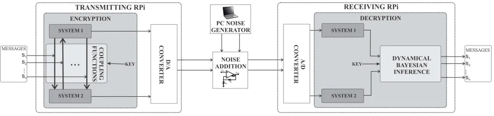
Fig. 1. Schematic of the realization of the coupling function communications protocol.
With these properties, coupling functions allow for the construction of an effective way of encrypting information transfer between dynamical systems. In particular, a set of linearly independent coupling functions between self-sustained dynamical systems can provide complex nonlinear mixing of the information, enabling a form of encryption that is very hard to break unless the exact coupling functions are known. As well as using coupled dynamical systems in this way, one can exploit further their dynamical properties to provide multiplexing and simultaneously yielding very noise robust communications.
The starting point of the enterprise was the time-varying, decomposable, coupling functions of the human cardiorespi-ratory interaction [28], [37]. Establishment of the nature of these biological coupling functions triggered the development of the communication protocol, which uses the same analysis methods developed for, and initially used on, the biological signals. The security of the protocol [21] is assured by use of multiple, time-varying, coupling functions between two or more dynamical systems, and the protocol inherently allows for the multiplexing of information. Of greatest interest in the present context is that the communication scheme is also highly noise-robust. The latter property results from the use of dynamical Bayesian inference for stochastic processes within the protocol, allowing effective separation between the deterministic information signals and the dynamical (channel) noise perturbations.
The previous theoretical and numerical foundations of the coupling function protocol are complemented here by the development of an experimental realization and the perfor-mance of robustness tests involving real analog noise. In the analog electronic experiments the states of the dynamical systems are truly continuous; measurement noise and other imperfections of the electronic components are unavoidable; and so the conditions are close to those of many real appli-cations [41]–[45]. Another aim of the experiment was to demonstrate the use of low-cost devices of the kind commonly available in general use (e.g. comparable to smart-phones and sensor network devices) [19], [20]. So we developed the transmitter and receiver on two Raspberry PI 2 single-board computers. Incorporating the analog signals and the appropriate electronic circuits, we then added analog electronic noise in order to simulate the reality of communications conditions. The robustness was then evaluated for different
levels of perturbing noise. The purpose of our new experiment was thus to test the capabilities and the limitations of the protocol when being applied under conditions similar to those that may be used in practice.
The paper is organized as follows. First we describe the main concepts in section II. These include a conceptual description of the implementation of the coupling function protocol, the specific dynamical systems in use and the method of dynamical Bayesian inference employed on the receiver side. Then in section III we give a detailed description and explanation of the analog electronic scheme and its components, followed by section IV presenting the signal analysis, taking account of the signals’ frequency content and establishing the effect of noise on the information transfer. Concluding remarks are given in section V. Finally, in the Appendix we demonstrate the effect of a low-frequency non-Gaussian noise on the communication protocol.
II. IMPLEMENTATION OFCOUPLINGFUNCTION
SECURECOMMUNICATION
This section describes the underlying principles of the method for secure communication, and their implementation. The protocol involves encryption of multiple information streams by using thm to scale the nonlinear coupling functions between dynamical systems; decryption involves dynamical Bayesian inference of the time-evolving parameters [21].
A. The Coupling Functions Protocol
The experimental communications system is illustrated in Fig. 1. A number of information carrying signals si, coming from different devices or channels, are to be trans-mitted simultaneously. Each signal serves as a scale parameter in the nonlinear coupling functions between two self-sustained systems in the transmitter. One signal from each of these is then transmitted through the public channel and, on the receiving side, is used for enslaving and completely synchro-nizing two similar coupled systems. Dynamical Bayesian inference is then applied, so that the model parameters can be inferred, allowing the information signals si to be decrypted.
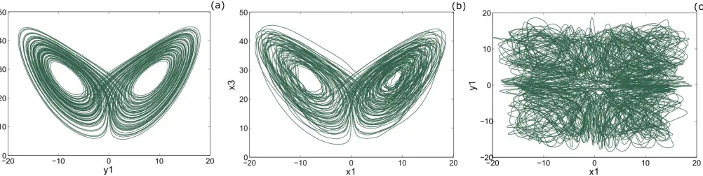
Fig. 2. The trajectories of the Lorenz systems used on the transmitting side: (a) The trajectories of y1 and y3 from the second autonomous Lorenz
system (Eq. (3)). The plot is as expected, with the trajectories attracted to stable points. (b) The trajectories of x1and x3from the first Lorenz system (Eq. (2)).
The graph is similar to the previous case, with a notable difference in the roughness of the trajectories. This is expected, and is a result of the fact that x1
contains the coupling elements. (c) The trajectories of x1and y1from both Lorenz systems during data transmission. The coupling Lissajous curve is chaotic
and it is evident that the solution is not contracted to a bounded and predictable trajectory space, but is instead well hidden in the chaotic and convoluted coupled trajectories and nonlinear dependences between the systems.
forms for the linearly independent coupling functions offers an unbounded number of possible combinations. The scheme facilitates multiplexing, and it is also very noise-robust because the Bayesian framework is by nature stochastic inference.
B. The Dynamical Systems Used
The basis of the encryption and decryption, and the model that is to be inferred, consists of two noisy M-dimensional interacting systems that can be described by the stochastic differential equation:
˙
xi =f(xi,xj|c)+
√
Dξi
=g(xi|c1)+q(xi,xj|c2)+
√
Dξi. (1)
Here, c is the parameter vector, f(xi,xj|c)are the base func-tions which describe the autonomous dynamics g(xi)and the coupling functions q(xi,xj),ξi is white Gaussian noise with autocorrelation< ξ(t)ξ(t) >=Dδ(t−t), and D is the noise diffusion matrix for white Gaussian noise, and i = j =1,2. For an analysis of the noise robustness of the protocol in the face of colored non-Gaussian noise, see the Appendix where the effect of a low-frequency Ornstein-Uhlenbeck process is considered. The dynamical systems used should be self-sustained, but in general need not be chaotic. However, chaotic systems offer an additional level of complexity (and hence security) for data encryption because they appear as random-like and unpredictable, even though their underlying nature is deterministic [46]. Furthermore, as discussed bellow, the attractors of chaotic coupled dynamical systems typically span a relatively large area in the state space, which is favourable for the Bayesian inference framework used for the decryption of the signals.
Ever since Lorenz came to appreciate the unusual charac-teristics of chaos [47] – in that the systems are deterministic in nature, but provide a random-like appearance – chaotic dynamical systems have been used widely in engineering, and in particular for secure communications [10], [11], [48]. The Lorenz chaotic system has been utilized extensively, partly
due to the nature of its attractor which spans a wide area in the state space (Fig. 2 (a)), and partly because it is quite stable and can withstand relatively high perturbations. In our experiment, a system of two coupled chaotic Lorenz systems was used, and two binary signals s1(t) and s2(t) therefore need to be transmitted. The first Lorenz system is given by
˙
x1=10x2−10x1+s1(t)cos(y1)x2+s2(t)x1y2/y3
˙
x2=28x1−x1x3−x2
˙
x3=x1x2−2.67x3; (2)
and the second one by
˙
y1 =10y2−10y1
˙
y2 =28y1−y1y3−y2
˙
y3 =y1y2−2.67y3. (3)
In x1 of the first oscillator, two coupling functions are
comprised of variables from both the first and more impor-tantly the second system. These two nonlinear coupling functions are just examples, and other choices of linearly independent functions can be used instead. The behavior of the systems can be seen in Fig. 2. The Lissajous curves show the relationships between two of the states in each system – Fig. 2 (a-b). The effect of the coupling on the first system shows up as relatively minor disturbances of its attractor Fig. 2 (b). The relationship between the mutually coupled states of the two systems during data transmission is shown in Fig. 2 (c). It demonstrates their complicated and convoluted inter-trajectories, which is the main property used for scrambling the information signals.
Only the signals x1and y2are then transmitted and noise is
added to them in the process of transmission. On the receiving side the two chaotic systems are completely synchronized [48]: the system u, through x1, becomes effectively identical to the
system x:
u1=x1
˙
u2=28x1−x1u3−u2
˙
and the system w, through y2, becomes effectively identical
to system y:
˙
w1 =10y2−10w1
w2 =y2
˙
w3 =w1y2−2.67w3. (5)
The time-series of the signals from the reconstructed dynam-ical systems u and w then act as the six inputs for the dynamical Bayesian inference.
C. Dynamical Bayesian Inference
Dynamical Bayesian inference for decryption of the signals si from the two reconstructed coupled systems u and w [21], [28] is performed in state space. The model that is to be inferred is given by Eq. (1). Note that the chosen coupling functions q(xi,xj) represent the encryption key. Bearing this in mind, if given a 2 × M time-series X = {xn ≡ x(tn)} (tn = nh) as input, the main task for the Bayesian dynamical inference is to reveal the unknown model parameters and the noise diffusion matrixM= {c,D}, which eventually comes down to maximization of the posterior conditional probability pX(M|X)of observing the parameters Mwhen given the dataX [49]. The relationship of this poste-rior conditional probability to the pposte-rior density ppposte-rior(M) (which encompasses observation based prior knowledge of the unknown parameters), and to the likelihood function(X|M) (that is the conditional probability density to observeX given choice M), is given by Bayes’ theorem:
pX(M|X)= (X|M)pprior(M)
(X|M)pprior(M)dM. (6) Using dense enough sampling h, the problem can be solved using the Euler midpoint x∗n=(xn+1+xn)/2 discretisation of Eq. (1):
xi,n+1=xi,n+h f(x∗i,n,x∗j,n|c)+h
√
Dzn. (7)
Here zn is the stochastic integral of the noise term over time:
zn≡
tn+1
tn z(t)dt. The noise znis statistically independent and
the likelihood is given by a product over n of the probability at each moment of time of observing xn+1. The joint probability
density of znis thus used to find the joint probability density of the process in respect of xn+1−xn. The negative log-likelihood
function S= −ln(X|M)is then expressed as:
S= N
2 ln|D| + h 2
N−1
n=0
ck∂f k(x·,n)
∂x
+ [˙xn−ckfk(x·∗,n)]T(D−1)[˙xn−ckfk(x·∗,n)]
, (8)
wherex˙n=(xn+1−xn)/h, with implicit summation over the repeated index k.
Given a multivariate normal distribution for the prior probability of the parameters c, with mean c, covariance matrix prior, and concentration matrix prior ≡−1prior, the posterior multivariate probabilityNX(c|¯c, )(and thus the probability density of each parameter set of the model (1)) can
be evaluated by applying the following four equations to each sequential block of dataX:
D= h
N
˙
xn−ckfk(x∗·,n)
T
˙
xn−ckfk(x∗·,n)
,
ck =(−1)kwrw,
rw =(prior)kwcw+h fk(x∗·,n) (D−1)x˙n± h 2
∂fk(x·,n)
∂x ,
kw =(prior)kw+h fk(x∗·,n) (D−1)fw(x∗·,n). (9) Here, summation over n = 1, . . . ,N is assumed, the initial prior is set to be the non-informative flat normal distribution given by prior = 0 and cprior¯ = 0, and summation over repeated indices k andwis implicit. The stopping rule is that further iteration of the algorithm would not modify c or beyond some predefined very small constant valueε.
The main concept of this approach is based on the fact that the inference has to follow the time evolution of c and, at the same time, to separate its dynamical effects from the unavoidable accompanying noise. For that purpose, the operations in Eqs. (9) are performed within a single window of data, where the time-series are separated into sequential blocks; the evaluation of each next block of data uses the evaluation results of the previous block, and the process of information propagation between the n posterior distribution and the n+1 prior distribution has to allow the time-variability of the parameters to be followed. A squared symmetric positive definite matrixdiffis created to show how much each parameter diffuses normally. Therefore, the next prior probability of the parameters is the convolution of two current normal multivariate distributions,post anddiff:
n+1
prior = npost+ndiff. The diffusion matrix is defined as (diff)i,j = ρi jσiσj, where σi is the standard deviation of the diffusion of ci in the current time window, andρi j is the correlation between the changes in the parameters ci and cj. Dynamical Bayesian inference is applied on the receiver side to the six time series (u1,u2,u3, w1, w2, w3) from the two reconstructed coupled systems to decrypt the binary signals s1(t) and s2(t). The base functions for the inference of the model within the Bayesian framework are taken as the functions on the right-hand sides of Eqs. (2) and (3).
Further details of the development, software implementation and application of the dynamic Bayesian inference approach can be found in [ [21], [27], [28], [49], and references therein.
III. ANALOGELECTRONICREALIZATION
Having summarised the basis of the theory, we now provide a detailed explanation of the practical experimental realization of this algorithm.
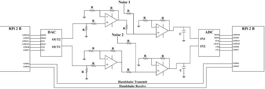
Fig. 3. Detailed scheme of the electronic implementation.
simulations to generate the signals in the transmitter and to reconstruct them in the receiver were performed using a fourth order Runge-Kutta scheme with a sampling of h=0.01.
The two random binary signals s1(t) and s2(t) generated in the transmitter were used as scale parameters in the nonlinear coupling functions between the systems given by Eqs. (2) and (3). Signals x1 and y2 were converted into
analog signals with a digital-to-analog convertor, amplified, and transmitted through wires to the receiver. While both signals were in their analog form, independent white noises were added to them. These noise signals were generated in Matlab and sent to the two independent analog outputs of a computer audio card with a 100 KHz sampling frequency. Both noise signals were of the same amplitude, and analysis of their mean, autocorrelation, and frequency spectra showed that they indeed possessed the characteristics of experimental white noise. Finally, on the receiving side, both analog signals were converted back to digital by an analog-to-digital convertor and then used to synchronize the chaotic systems in the receiver, as shown in Eqs. (4) and (5). Both converters were implemented with ‘ADC-DAC Pi’ cards. These cards are based on the Microchip MCP3202 ADC converter containing 2 analog inputs with 12 bit resolution and a Microchip MCP4822 dual channel 12-bit DAC with an internal voltage reference. General purpose quad operational amplifiers TL084N were used, along with standard resistors and capacitors, as shown in Fig. 3.
The logic of the transmission included a handshake with direct digital input/output connections between the two Raspberry PIs (indicated by the two lines on the bottom of Fig. 3). This involved the transmitter sending a digital binary indication that it is ready to transmit, and then the receiver returning a bit to indicate that it is ready to receive. As speed of the communication was not the focus in this inves-tigation, the time window in which the Bayesian inference was applied was 250 s, i.e. each bit {0 or 1} was transmitted within this window length.
[image:5.612.335.537.273.439.2]Fig. 4 shows samples of the three signal time-series captured by an oscilloscope at an arbitrary time. The bottom signal is the transmitted analog signal y2(t); the middle signal is the
Fig. 4. Real-time oscilloscope capture of the transmitted signal y2(t)
(bottom), the white noise (middle), and the same signal y2(t)but with added
noise that arrives at the receiver (top).
added analog white noise; while the top signal is y2(t)after the noise addition. This top trace demonstrates the effect of the white noise on the generated audio signal(s) i.e. on the transmitted information.
IV. ANALYSIS
A. Time and Frequency Signal Analysis
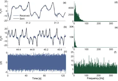
Fig. 5. Time-series analysis of the transmitted, the received and the noise signals and their corresponding FFT spectra: (a) Time-series of the received, reconstructed, signal x1(t)superimposed on its original transmitted version. (b) Time-series of the received signal y2(t)superimposed on its original transmitted
version. (c) The discretized analog white noise time-series. (d) The FFT frequency spectrum of x1(t). (e) The FFT frequency spectrum of y2(t). (f) The FFT
frequency spectrum of the noise signal.
Fig. 6. Deviations of the decrypted signal from the initial binary states due to noise, presented as compact box plots (in terms of descriptive statistics: median, quartiles, max, and min) as a function of signal-to-noise ratio (SNR). (a) For the first information signal s1(t)i.e. inferred parameter c1where the
binary value for {1} is represented by c1=2.7, and (b) for the signal s2(t)i.e. inferred parameter c2with the binary {1} represented by c2=1.5.
contained all frequencies, spread across the entire observed domain, as expected for a white noise process.
B. Influence of Noise on Information Transfer
The main goal of the experiment was to test the effec-tiveness and robustness of coupling function encryption for communication in the presence of noise, and thus to examine its practical applicability. The second part of the investigation therefore consisted of systematically increasing the strength of the noise while, at the same time, following its effect on the
signal-to-noise ratio (SNR). Randomly generated bits {0,1} were transmitted while gradually increasing the noise level (decreasing the SNR) in each trial. Fig. 6 shows the deviations of the binary 1 and binary 0 decrypted signal s1(t) (i.e. the inferred parameter c1), and signal s2(t) (i.e. the inferred
parameter c2) as functions of the SNR. Thus for each SNR
point examined there was one trial of transmission and the parameters c1 and c2 are plotted as two boxplots (showing
[image:6.612.54.558.390.554.2]The encryption/decryption was performed down to around SNR=15 dB for the two simultaneous parameters c1and c2,
after which the experiment became impossible (most probably due to experimental limitations and the 12-bit resolution of the DAC and ADC). The experimental setup increased the SNR threshold at which a finite BER appeared, cf. the SNR=4 dB obtained in theory and through numerical simulations [21]. With the encryption/decryption of only the first parameter c1,
effective communication was performed for SNR=14.1 dB. Thus for this SNR, which is below 15 dB, there was no BER and reliable communication was possible. This is a rela-tively high level of noise (i.e. low SNR) for communications in practice, where the SNR threshold for finite BER is around 15 dB for wireless transmission and around 40 dB for wireline communication [50].
In order to establish the effectiveness of the coupling func-tion protocol, it was compared with a known protocol based on complete synchronization of chaotic dynamical systems called the signal masking protocol [10]. The latter is one of the most used protocols in the class of secure communications with (chaotic) dynamical systems, so that this test is representative and relevant to all protocols in this class. Because the protocol presented in this paper also uses complete synchronization to transmit the signals, this investigation also tests how coupling function communication behaves in a noisy commu-nications environment without dynamical Bayesian inference. In comparison, the signal masking protocol, which relies only on complete synchronization, is less complex than the coupling function protocol which uses complete synchronization plus dynamical Bayesian inference for decryption and noise reduc-tion. This complexity implies a need for higher computational power and associated lower speed in the case of coupling function communications. In order to achieve a meaningful comparison, the same number of random bits were transmitted within same window length, using the same hardware setup, systematically applying the same noise levels i.e. SNR. It was found that a finite BER appeared at around SNR = 20 dB, which is a significantly higher threshold (thus indicating lower robustness) than the values of SNR =14.1 dB and SNR = 15 dB obtained with the coupling function protocol.
V. CONCLUSION
The communications protocol encrypted the information through the complex nonlinear mixing provided by the mech-anisms of interaction defined by coupling functions. Here we presented a simple experimental proof of concept, testing the noise robustness of the protocol under realistic conditions. Thus, the work has developed the engineering aspects of the previous theoretical concepts.
(as GPU or FPGA for example), which in turn would allow for higher bit conversion-rates than the 12-bit resolution used here. The use of complete synchronization is not easy to maintain in practice where the transmitter and receiver are sufficiently widely separated, in which case one should apply one of the known methods for maintaining data synchroniza-tion in communicasynchroniza-tion networks [51], [52]. In theory, the noise acted as dynamic perturbation of the dynamical states, but in the experiments here we also encountered a small amount of measurement noise, making the inference less precise. Future calculations of the inference should employ one of the known procedures for decomposing the measurement noise as well.
The coupling function protocol was shown experimentally to remain effective even with relatively high noise. All of the results were consistent with the earlier theoretical findings and demonstrated that the protocol could with advantage be employed in current communications applications, in partic-ular when noise levels are high. Dynamical Bayesian inference for stochastic processes was shown to be useful in decom-posing the noise from the deterministic information. In the present case, this was valuable in relation to the coupling function protocol, but it also promises future applications to noise reduction in communications using other protocols.
APPENDIX
ANALYSIS OF THEINFLUENCE OFLOW-FREQUENCY
NON-GAUSSIANNOISE ON THEINFORMATIONTRANSFER
The interference that arises in communications networks is often modeled as a Gaussian random process to which the central limit theorem is applicable. This can be appropriate when the noise is caused by different mutually independent and uncorrelated signals, none of which dominates their total accumulation. A notable example is the thermal noise in elec-tronics, which can be modeled as additive white Gaussian noise. However, there are many real-world situations where dominant sources of interference occur, often as the result of distance-dependent path-loss attenuation [53]. In such cases, the central limit theorem cannot give a satisfactory approxima-tion, because the probability density function of the interfer-ence features a heavier tail than that predicted by the Gaussian model. Models that have been proposed for such interfer-ence include the Ornstein-Uhlenbeck process [54], [55], 1/f noise [56], the spatial Poisson process [57], and Gaussian mixture models.
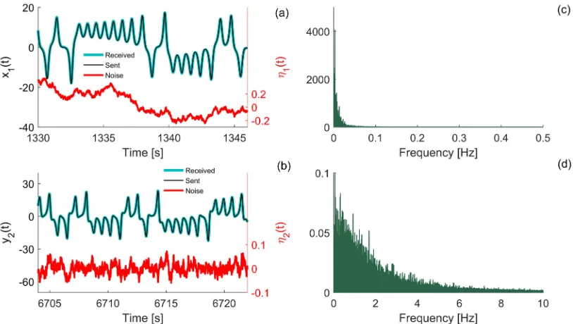
Fig. 7. Time-series analyses of the transmitted and received signals, and of the noise signals and their corresponding FFT spectra. (a) Time-series of the received signal x1(t)superimposed on its original transmitted version with Ornstein-Uhlenbeck noise η1(t)of strength D1 =20 and correlation time
γ1 =30 (red trace, and right-hand ordinate axis) is applied. (b) Time-series of the received signal y2(t)superimposed on its original transmitted version
with Ornstein-Uhlenbeck noise η2(t)of strength D2=20 and correlation timeγ2=0.09 (red trace and right-hand ordinate axis) is applied. (c) The FFT
frequency spectrum ofη1(t). (d) The FFT frequency spectrum ofη2(t). Note thatη2(t)has a short correlation time and is thus looks more like white noise
thanη1(t), which can seen in both the time evolutions and the frequency spectra.
Ornstein-Uhlenbeck noise η(t)was added to the sent signals
x1and y2from the coupled systems given in (2) and (3). Thus,
during the simulated transmission we have x1 =x1+η1(t)
and y2 = y2+η2(t), where η1(t) and η2(t) are
Ornstein-Uhlenbeck noise signals that influence the respective channels. In general, Ornstein-Uhlenbeck noise can be defined as:
˙
η(t)=ξ(t)− 1
γη(t), (10)
with autocorrelationη(t)η(t) =σ2exp[−(t−t)/γ]. Here, ξ is white Gaussian noise and γ is the correlation time of the random Ornstein-Uhlenbeck process. For the limiting case where γ → 0, the random process converges to white Gaussian noise. In reality however, the noise often has a nonzero correlation time that cannot be neglected. The Ornstein-Uhlenbeck process is one such natural gener-alization of Gaussian white noise, and it can be used to represent the noise that occurs in real-world communication systems [58]. It is a mean-reverting process, which means that it does tend to drift towards a long-term mean over time; however, during the relatively brief time windows in which communication occurs (both in reality and in the simulation), and for long enough values of the correlation time, this tendency can be neglected and the noise can be treated as being distinctively different from standard Gaussian white noise.
By definition the Ornstein-Uhlenbeck process is Gaussian in the stationary limit. However, before the stationary limit is reached, for example for short time periods comparable with the communication bit time-length, the Ornstein-Uhlenbeck process can be regarded as being non-Gaussian. The noise
signals generated with (10) were therefore subjected to both the Kolmogorov-Smirnov and the Anderson-Darling tests in order to examine the similarity of their distributions to the standard normal distribution. Both tests showed that, for the time windows used here, and for the correlation times
γ ≥0.09, the generated noises do not come from a Gaussian distribution.
Numerical simulations with Ornstein-Uhlenbeck noise applied to the communication channel were run for times of 20,000 seconds, during which 400 data bits were sent and decrypted over 400 Bayesian windows of 50 seconds each, while the sampling time was 0.01 seconds. Fig. 7 shows the time-series of the transmitted and the received signals for both x1(t) and y2(t). It also gives the time-series and the corresponding FFT power spectra for the noise. The noise signalη1(t)applied to x1(t)had a strength of D1=
20 and a correlation time of γ1 = 30. As can be seen in Figs. 7(a) and (c) respectively, the longer correlation time meant a more visible drift of the noise within the time domain and a power spectrum restricted to much lower frequencies, confirming the nature of the Ornstein-Uhlenbeck process as a model of a low-pass-filtered white noise. On the other hand, the noise signalη2(t)applied to y2(t)had the same strength of D2=20, but a much shorter correlation time ofγ2=0.09,
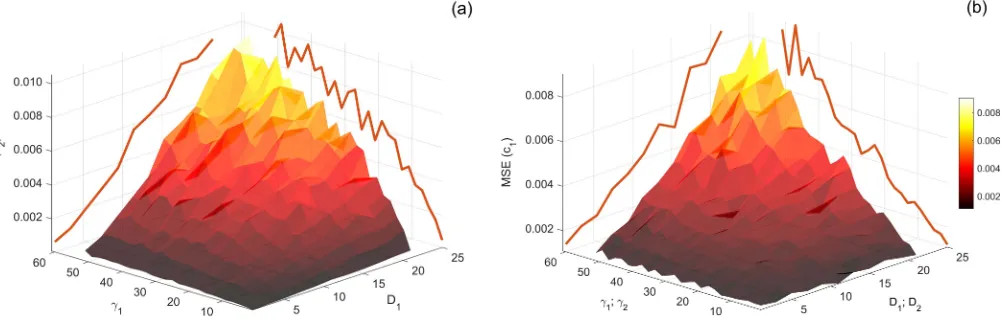
Fig. 8. The dependance of the mean-square error (MSE) of the transmitted bits on the strength D and correlation timeγ of the Ornstein-Uhlenbeck noise applied to the communication channels. (a) The mean-square error of c2(t)as a function of D1 andγ1 of the noise signalη1(t)applied to x1(t), while
the parameters of the noise applied to y2 remain constant. The mean-square error increases with the strength and correlation time of the noise. (b) The
mean-square error of c1(t)as a function of D1andγ1, and of D2andγ2, of the noise signalsη1(t)applied to x1(t)andη2(t)applied to y2(t), respectively.
Again, the mean-square error increases with the strengths and the correlation times of the noise signals.
correlation time can effectively transform the generated noise from a white Gaussian one into a low-frequency one.
Fig. 8 shows how successful the dynamical Bayesian inference was in dealing with noise of this nature, using the mean-square error between the sent and the received values of the decrypted bits c1(t) and c2(t): M S E(c) =
1
n
n
i=1(cdecrypted−csent)2. First, simulations were run where
the parameters of η2(t)were kept at constant values of D2= γ2 = 1, while the parameters of η1(t) were being changed in the ranges of[0;22]for D1and of[0;52]forγ1. The
mean-square error of the decrypted bit c2(t) was then calculated for each of the simulation scenarios and plotted as a func-tion of D1 and γ1. In Fig. 8(a), it can be seen that this
error increases as either the noise strength or the correlation time increases. Furthermore, the projections of the three-dimensional surface on the side plains show that the error rises more steadily and linearly with the increase of D1, than
it does with the increase ofγ1. Similar plots were obtained for the dependance of the mean-square error of the bit c1(t)on the change of the parameters ofη1(t), and for the dependance of the mean-square errors of both c1(t)and c2(t)on the change of the parameters ofη2(t). These plots have been omitted in view of space considerations.
Another situation that was simulated was the simultaneous increase in the strength and correlation time of both noise signalsη1(t)andη2(t). As can be seen in Fig. 8(b), the mean-square error of the decrypted bit c1(t) also rises with the increase of these parameters. Again, the change of the noise strengths contributes towards a steadier and more linear-like increase than the change of the correlation times. Similar results were obtained for the dependence of the mean-square error of c2(t)on the change of the noise parameters.
In summary, the framework for dynamical Bayesian infer-ence (itself stochastic by nature) is, by construction, better capable of dealing with noise in the communication channel
that resembles Gaussian noise (i.e. has a shorter correlation time), but we find that it also exhibits satisfactory performance when more realistic forms of noise, such as low-frequency Ornstein-Uhlenbeck noise, are applied.
ACKNOWLEDGMENT
The authors are grateful to Robert J. Young for helpful discussions.
REFERENCES
[1] C. E. Shannon, “Communication theory of secrecy systems,” Bell Labs
Tech. J., vol. 28, no. 4, pp. 656–715, Oct. 1949.
[2] C. E. Shannon, “Communication in the presence of noise,” Proc. Inst.
Radio Eng., vol. 37, no. 1, pp. 10–21, Jan. 1949.
[3] P. C. Pinto, J. Barros, and M. Z. Win, “Secure communication in stochastic wireless networks—Part I: Connectivity,” IEEE Trans. Inf.
Forensics Security, vol. 7, no. 1, pp. 125–138, Feb. 2012.
[4] M. Ozmen and M. C. Gursoy, “Secure transmission of delay-sensitive data over wireless fading channels,” IEEE Trans. Inf. Forensics Security, vol. 12, no. 9, pp. 2036–2051, Sep. 2017.
[5] H. Gou, A. Swaminathan, and M. Wu, “Intrinsic sensor noise features for forensic analysis on scanners and scanned images,” IEEE Trans. Inf.
Forensics Security, vol. 4, no. 3, pp. 476–491, Sep. 2009.
[6] J. Lukäš, J. Fridrich, and M. Goljan, “Digital camera identification from sensor pattern noise,” IEEE Trans. Inf. Forensics Security, vol. 1, no. 2, pp. 205–214, Jun. 2006.
[7] H. Zhao and Y. Q. Shi, “Detecting covert channels in computer networks based on chaos theory,” IEEE Trans. Inf. Forensics Security, vol. 8, no. 2, pp. 273–282, Feb. 2013.
[8] C. E. Shannon, “A mathematical theory of communication,” Bell Syst.
Tech. J., vol. 27, no. 3, pp. 379–423, Jul./Oct. 1948.
[9] L. B. Kish, “Totally secure classical communication utilizing Johnson (-like) noise and Kirchoff’s law,” Phys. Lett. A, vol. 352, no. 3, pp. 178–182, 2006.
[10] K. M. Cuomo and A. V. Oppenheim, “Circuit implementation of synchronized chaos with applications to communications,” Phys. Rev.
Lett., vol. 71, pp. 65–68, Jul. 1993.
[11] L. Kocarev and U. Parlitz, “General approach for chaotic synchroniza-tion with applicasynchroniza-tions to communicasynchroniza-tion,” Phys. Rev. Lett., vol. 74, no. 25, pp. 5028–5031, 1995.
[13] G. Kaddoum, E. Soujeri, and Y. Nijsure, “Design of a short refer-ence noncoherent chaos-based communication systems,” IEEE Trans.
Commun., vol. 64, no. 2, pp. 680–689, Jan. 2016.
[14] N. Li, J.-F. Martínez-Ortega, V. H. Díaz, and J. M. M. Chaus, “A new high-efficiency multilevel frequency-modulation different chaos shift keying communication system,” IEEE Systems J., to be published, doi:10.1109/JSYST.2017.2715661.
[15] Y.-Z. Liu et al., “Exploiting optical chaos with time-delay signature suppression for long-distance secure communication,” IEEE Photon. J., vol. 9, no. 1, pp. 1–12, Feb. 2017.
[16] C. H. Bennett, “Quantum information and computation,” Nature, vol. 404, no. 6775, pp. 247–255, 2000.
[17] K. A. Patel et al., “Coexistence of high-bit-rate quantum key distribution and data on optical fiber,” Phys. Rev. X, vol. 2, no. 4, p. 041010, 2012. [18] M. F. Haroun and T. A. Gulliver, “Secret key generation using chaotic signals over frequency selective fading channels,” IEEE Trans. Inf.
Forensics Security, vol. 10, no. 8, pp. 1764–1775, Aug. 2015.
[19] H.-G. Chou, C.-F. Chuang, W.-J. Wang, and J.-C. Lin, “A fuzzy-model-based chaotic synchronization and its implementation on a secure communication system,” IEEE Trans. Inf. Forensics Security, vol. 8, no. 12, pp. 2177–2185, Dec. 2013.
[20] D. Irakiza, M. E. Karim, and V. V. Phoha, “A non-interactive dual channel continuous traffic authentication protocol,” IEEE Trans. Inf.
Forensics Security, vol. 9, no. 7, pp. 1133–1140, Jul. 2014.
[21] T. Stankovski, P. V. E. McClintock, and A. Stefanovska, “Coupling func-tions enable secure communicafunc-tions,” Phys. Rev. X, vol. 4, p. 011026, Feb. 2014.
[22] T. Stankovski, T. Pereira, P. V. E. McClintock, and A. Stefanovska, “Coupling functions: Universal insights into dynamical interaction mechanisms,” Rev. Mod. Phys., vol. 89, no. 33, p. 045001, 2017. [23] A. Pikovsky, M. Rosenblum, and J. Kurths, Synchronization: A
Universal Concept in Nonlinear Sciences. Cambridge, U.K.: Cambridge
Univ. Press, 2001.
[24] M. G. Rosenblum and A. S. Pikovsky, “Detecting direction of coupling in interacting oscillators,” Phys. Rev. E, Stat. Phys. Plasmas Fluids Relat.
Interdiscip. Top., vol. 64, no. 4, p. 045202, 2001.
[25] B. Kralemann et al., “In vivo cardiac phase response curve elucidates human respiratory heart rate variability,” Nature Commun., vol. 4, Sep. 2013, Art. no. 2418.
[26] I. T. Tokuda, S. Jain, I. Z. Kiss, and J. L. Hudson, “Inferring phase equations from multivariate time series,” Phys. Rev. Lett., vol. 99, p. 064101, Aug. 2007.
[27] V. N. Smelyanskiy, D. G. Luchinsky, A. Stefanovska, and P. V. E. McClintock, “Inference of a nonlinear stochastic model of the cardiorespiratory interaction,” Phys. Rev. Lett., vol. 94, no. 9, p. 098101, 2005.
[28] T. Stankovski, A. Duggento, P. V. E. McClintock, and A. Stefanovska, “Inference of time-evolving coupled dynamical systems in the presence of noise,” Phys. Rev. Lett., vol. 109, no. 2, p. 024101, 2012.
[29] J. T. C. Schwabedal and A. Pikovsky, “Effective phase dynamics of noise-induced oscillations in excitable systems,” Phys. Rev. E, Stat. Phys.
Plasmas Fluids Relat. Interdiscip. Top., vol. 81, no. 4, p. 046218, 2010.
[30] Z. Levnaji´c and A. Pikovsky, “Network reconstruction from random phase resetting,” Phys. Rev. Lett., vol. 107, p. 034101, Jul. 2011. [31] I. Z. Kiss, C. G. Rusin, H. Kori, and J. L. Hudson, “Engineering
complex dynamical structures: Sequential patterns and desynchroniza-tion,” Science, vol. 316, no. 5833, pp. 1886–1889, 2007.
[32] J. Miyazaki and S. Kinoshita, “Determination of a coupling function in multicoupled oscillators,” Phys. Rev. Lett., vol. 96, p. 194101, May 2006.
[33] I. Z. Kiss, Y. Zhai, and J. L. Hudson, “Predicting mutual entrainment of oscillators with experiment-based phase models,” Phys. Rev. Lett., vol. 94, p. 248301, Jun. 2005.
[34] T. Stankovski, V. Ticcinelli, P. V. E. McClintock, and A. Stefanovska, “Coupling functions in networks of oscillators,” New J. Phys., vol. 17, no. 3, p. 035002, 2015.
[35] T. Stankovski, S. Petkoski, J. Raeder, A. F. Smith, P. V. E. McClintock, and A. Stefanovska, “Alterations in the coupling functions between cortical and cardio-respiratory oscillations due to anaesthesia with propofol and sevoflurane,” Philos. Trans. Roy. Soc. London A, Math.
Phys. Sci., vol. 374, no. 2067, p. 20150186, 2016.
[36] T. Stankovski, V. Ticcinelli, P. V. E. McClintock, and A. Stefanovska, “Neural cross-frequency coupling functions,” Front. Syst. Neurosci., vol. 11, p. 33, Jun. 2017, doi:10.3389/fnsys.2017.00033.
[37] D. Iatsenko et al., “Evolution of cardiorespiratory interactions with age,”
Philos. Trans. Roy. Soc. London A, Math. Phys. Sci., vol. 371, no. 1997,
p. 20110622, 2013.
[38] B. Kralemann, L. Cimponeriu, M. Rosenblum, A. Pikovsky, and R. Mrowka, “Phase dynamics of coupled oscillators reconstructed from data,” Phys. Rev. E, Stat. Phys. Plasmas Fluids Relat. Interdiscip. Top., vol. 77, no. 6, p. 066205, 2008.
[39] S. Ranganathan, V. Spaiser, R. P. Mann, and D. J. T. Sumpter, “Bayesian dynamical systems modelling in the social sciences,” PLoS ONE, vol. 9, no. 1, p. e86468, 2014.
[40] T. Stankovski, A. Stefanovska, R. J. Young, and P. V. E. McClintock, “Encoding data using dynamic system coupling,” U.S. Patent 0 182 220 A1, Jun. 23, 2016.
[41] D. G. Luchinsky, P. V. E. McClintock, and M. I. Dykman, “Analogue studies of nonlinear systems,” Rep. Prog. Phys., vol. 61, no. 8, pp. 889–997, 1998.
[42] U. Parlitz, L. Junge, W. Lauterborn, and L. Kocarev, “Experimental observation of phase synchronization,” Phys. Rev. E, Stat. Phys.
Plasmas Fluids Relat. Interdiscip. Top., vol. 54, pp. 2115–2117,
Aug. 1996.
[43] T. Stankovski, P. V. E. McClintock, and A. Stefanovska, “Dynamical inference: Where phase synchronization and generalized synchronization meet,” Phys. Rev. E, Stat. Phys. Plasmas Fluids Relat. Interdiscip. Top., vol. 89, no. 6, p. 062909, 2014.
[44] G. Millérioux, J. M. Amigó, and J. Daafouz, “A connection between chaotic and conventional cryptography,” IEEE Trans. Circuits Syst. I,
Reg. Papers, vol. 55, no. 6, pp. 1695–1703, Jul. 2008.
[45] K. M. Cuomo, A. V. Oppenheim, and S. H. Strogatz, “Synchronization of Lorenz-based chaotic circuits with applications to communications,”
IEEE Trans. Circuits Syst. I, Fundam. Theory Appl., vol. 40, no. 10,
pp. 626–633, Oct. 1993.
[46] J. P. Crutchfield, “Between order and chaos,” Nature Phys., vol. 8, no. 1, pp. 17–24, 2012.
[47] E. N. Lorenz, “Deterministic non-periodic flow,” J. Atmos. Sci., vol. 20, no. 6, pp. 130–141, 1963.
[48] L. M. Pecora and T. L. Carroll, “Synchronization in chaotic systems,”
Phys. Rev. Lett., vol. 64, no. 8, pp. 821–824, 1990.
[49] T. Stankovski, A. Duggento, P. V. E. McClintock, and A. Stefanovska, “A tutorial on time-evolving dynamical Bayesian inference,” Eur.
Phys. J. Special Topics, vol. 223, no. 13, pp. 2685–2703, 2014.
[50] G. Alvarez and S. Li, “Some basic cryptographic requirements for chaos-based cryptosystems,” Int. J. Bifurcation Chaos, vol. 16, no. 8, pp. 2129–2151, 2006.
[51] D. J. Worsley and B. C. Edem, “Method of maintaining frame synchronization in a communication network,” U.S. Patent 5 668 811 A, Sep. 16, 1997.
[52] C. Halim and J. W. Stossel, “Remote data access and synchronization,” U.S. Patent 6 304 881 B1, Oct. 16, 2001.
[53] H. ElSawy, A. Sultan-Salem, M. S. Alouini, and M. Z. Win, “Modeling and analysis of cellular networks using stochastic geometry: A tutorial,” IEEE Commun. Surveys Tuts., vol. 19, no. 1, pp. 167–203, 1st Quart., 2017.
[54] P. Hanggi, T. J. Mroczkowski, F. Moss, and P. V. E. McClintock, “Bistability driven by colored noise: Theory and experiment,” Phys.
Rev. A, Gen. Phys., vol. 32, pp. 695–698, Jul. 1985.
[55] C. W. Gardiner, Handbook of Stochastic Methods. New York, NY, USA: Springer, 2004.
[56] P. Bak, C. Tang, and K. Wiesenfeld, “Self-organized criticality: An explanation of the 1/f noise,” Phys. Rev. Lett., vol. 59, pp. 381–384,
Jul. 1987.
[57] M. Z. Win, P. C. Pinto, and L. A. Shepp, “A mathematical theory of network interference and its applications,” Proc. IEEE, vol. 97, no. 2, pp. 205–230, Feb. 2009.
acquisition systems in large civil engineering projects. He has been a member of international collaborative projects (Skills Development for Young Researchers and Educational Personnel in Nano and Microelectronics Curricula and Microelectronics Cloud Alliance) for the introduction and development of study programs for microelectromechanical and nanoelectro-mechanical systems in Macedonian universities.
His research interests include the fields of network control systems, nonlinear control, noise robustness, secure communications, decentralized state estimation, machine learning, and work with big data.
Matej Dobrevski received the M.Sc. degree from
the Faculty of Electrical Engineering and Infor-mation Technologies, Ss Cyril and Methodius University in Skopje, Macedonia, in 2014. He is currently pursuing the Ph.D. degree with the Faculty of Computer and Information Science, Ljubljana, Slovenia. He was a Teaching and Research Assistant with Ss Cyril and Methodius University in Skopje.
His research interests include reinforcement learning and active vision.
Christopher Anderson was born in Greater Manchester, U.K., in 1967. He received the B.Sc. degree (Hons.) in applied physics with electronics from the University of Salford in 1990 and the Ph.D. degree in high energy physics from the University of Liverpool in 1999 (Application of Gigabit Links for use in High Energy Physics Trigger Processing for the Atlas project on the LHC at CERN).
Since 1990, he has held several industrial positions that combine interests in physics and electronics, including the design and development of hardware, software and complex electronic hardware (field programmable gate arrays) for physics research, defence, aerospace, and nuclear and comms. He has held several senior positions, including Chief Software Engineer and Design Authority for defence, aerospace, and naval projects, a Lead Engineer for safety related aerospace projects, the Principal EC&I Engineer for nuclear fusion and fission projects, and a Reactor Lead for the Generic Design Assessment of C&I for a candidate reactor for nuclear new build, reporting to the Office for Nuclear Regulation. He currently runs his own business, as a Functional Safety Consultant in Greater Manchester.
Dr. Anderson holds memberships and charterships as follows: CPhys, CEng, MInstP, and MIET. He is also an Honorary Research Associate at the University of Lancaster, Physics and Engineering Departments.
a Lecturer in 1970, a Senior Lecturer in 1979, a Reader in 1983, and he was appointed as a Professor of physics in 1991. He is currently a Research Professor Emeritus in physics. His research interests include superfluidity, quantum turbulence, fluctuation theory, chaos, and nonlinear dynamics, including phenomena and applications in living systems.
Dr. McClintock is a fellow of the Institute of Physics, U.K., where he is also a Chartered Physicist.
Aneta Stefanovska received the Ph.D. degree from
the University of Ljubljana, Slovenia, in 1992, working in part at the University of Stuttgart, Germany.
She is currently a Professor of biomedical physics and the Head of the Nonlinear and Biomedical Physics Group, Physics Department, Lancaster University, U.K. She has extensive experience in studying the physics of living systems combining measurements, time-series analyses, and modeling based on the phase dynamics approach. She has pioneered several new approaches to the analysis and modeling of time-varying oscillatory dynamical systems with applications to oscillatory cardiovascular, brain, and cell dynamics. Her particular interest is in non-autonomous dynamics of living systems.
Mile Stankovski received the Ph.D. degree from Ss
Cyril and Methodius University in Skopje, Mace-donia, in 1997. He was with the University of Woolverhampton, U.K.
He is currently a Professor of automation, system engineering and robotics and the Head of the Insti-tute of Automation and System Engineering with the Faculty of Electrical Engineering and Informa-tion Technology, UKIM, Macedonia. He has almost 20 years of industrial experience and has been employed in a number of applicative and scientific projects. He has extensive experience in industrial process control, networked control, robotics, and also in water and waste water system control.
Tomislav Stankovski received the B.S. degree
from the Faculty of Electrical Engineering and Information Technologies, Ss Cyril and Methodius University in Skopje, Macedonia, in 2008, and the Ph.D. degree from the Physics Department, Lancaster University, U.K., in 2012. He was a Research Associate at Lancaster University until 2014.