Generation and Analyzes of Guided WAVES in Planar Structures

Engineering,2011, 3, 532-537

doi:10.4236/eng.2011.35062 Published Online May 2011 (http://www.scirp.org/journal/eng)

Generation and Analyses of Guided Waves in

Planar Structures

Enkelejda Sotja1_{, P. Malkaj}2_{, Dhimiter Sotja}2

1_{Department of Manufacturer-Management, Polytechnic University of Tirana, Tirana, Albania} 2_{Department of Mechanics, Polytechnic Uni ersity of Tiranav , Tirana, Albania}

E-mail: [email protected],[email protected]

ReceivedFebruary 11, 2011; revised March 22, 2011; accepted April 8, 2011

Abstract

Guided wave in plate propagates like shear waves and Lamb waves. Both kinds are very dispersive waves. Generation and analysis of dispersion curves is very important. Those are used to predict and describe the relation between frequency, thickness with phase velocity, group velocity and wave mode. For a stainless steel plate with thickness 5.89 mm we built dispersion curves for shear and Lamb waves. A method based on peak frequency shifts of the shear waves along with the thickness was applied. In line with dispersion curves of shear waves phase velocity was seen that mode of waves translate in some points, have experiment per-formance much better than other points.

Keywords:Guided Wave, Dispersion Curves, Shear Wave, Lamb Wave

1. Introduction

Low frequency ultrasonic waves propagate in long dis-tance in the league (meters compared to millimeters in conventional techniques in UT), with small loss of en-ergy, which are called “directed waves” (guided wave).

Guided waves monitor large areas from a single posi-tion even when the objects are not fully physically ac-cessible, and they propagate standing localized between surfaces of a thin-walled structure, and even it is curved. These properties make them important for the ultrasonic control of facilities of special importance as airplanes, helicopters, spaceship, pressure vessels, and oil deposits. A very important use of guided waves is in the control of oil and gas pipelines and heat city systems regardless of their underground or underwater location [1].

Guided waves are cited as elastic waves that propagate in the samples where the axial dimension is many times greater than the dimensions of the section. The energy of these waves is guided from the boundaries of the sample with the environment, or other materials [2].

For each object’s form and for any combination of dimensions (e.g. section size or the internal and external diameter), there is now a unique set of wave dissemina-tion or the wave’s mode. Any one of these wave’s mode will be propagate with a set pattern, known as the shape of the mode [3].

The changing of the wave mode frequency is

associ-ated with the change of shape of the mode, phase’s ve-locity, group’s velocity. In order to predict the relation between frequency, the thickness of the structure and other parameters mentioned above there are used disper-sion curves (so called because the change of the fre-quency brings the change of wave velocity and vibra-tions tent to disperse during the spread). The data in these curves are used to do the tests controlling the structures, ranging from defining the generating equip-ment parameters of the guided waves in the structures until the final calculations [4].

2. Overview of the Propagation of the

Guided Waves in the Plan Structures

The simple forms of ultrasonic guided waves in plan structures are shear (transversal) waves. Movement of particles to the shear wave polarized parallel to the sur-face of the flat structure and perpendicular to the direc-tion of the spread of the wave. Shear waves appear symmetrical or asymmetrical. All modes are dispersive with exception of the base mode of the spread.

Lamb waves are guided waves the most complicated ones that propagate in a structure. Lamb waves propagate according to two basic wave mode, symmetric Lamb wave S0, S1, S2, and non-symmetric Lamb wave A0, A1,

A2, both are dispersive types. Greater value of f ·d causes

si-multaneously. For small values of the product f·d may exist only the basic mode Lamb wave (symmetrical and asymmetrical S0, A0) [5].

3. Spread of the Guided Wave Run in Plate

Structures (Mathematical Formalism)

In an elastic isotropic environment, waves propagate freely in all directions. Using the 3D elasticity theory in which the vector equation of the movement according Navier’s equations is [6]:



_{ }

 

_{  u}



_{  } 2_{u u (1)} λ and μ are Lame constants, ρ is mass density, and u is the displacement vector. Displacement vector in solid bodies is given in function of the two potential functions, a scalar potential Φ and a vector potential

x y z

H H H

  

H i j k which is known as Helmholtz’

solution,

   

u   H (2)

Rewrite the vector equation of movement by using the Equation (2), it is benefited the equation of the wave for potential scalar function Φ and vector potential H.

2 2 2 2 p s c c H          H  (3)

where the potential scalar propagates with cp,

longitudi-nal wave speed, and vector potential propagate with cs,

shear wave speed.

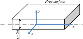
Recognize 3-D waves with straight crested. In straight- crested waves, the wave front is parallel to the axis z and the wave spread along z does not change (Figure 1). All the functions included in the analysis do not depend on z and the normal wave front will be perpendicular to the axis z, nk where k is the unit vector of z axis so,

0 and

z x

 _{ }  _

  i j y



[image:2.595.75.282.520.708.2]

 (4)

Figure 1. z-invariant plane of 3Dwaves.

Replacement of Equation (4) to (2) shows that dis-placement has components in all three directions (x, y, z),

Z Z Y

H H H H_X

x y y x x

 

      

 _  _ _  _ _ 

     

    

u i j k

y

 

 (5) The equation of wave for potentials scalar function Φ, Hx, Hy, Hz which satisfy the above conditions become,

2 2

2 2 2 2

2 2

0

S x x

y

x z

p S y y

S z z

c H H

H

H H

c c H H

x y z

c H H

                            (6)

For a plate sample with upper and lower surface without tension, set y = ±d (Figure 2), lied to infinity in directions x and z, government equations which satisfy the scalar and vector potential functions of the waves are,

2 2

2 2

2 2 2 2

1 1

, dhe

p s

c  c 

  

0

      

 

H

H  H (7)

Replacement in these governing equations the scalar and vector functions of the wave (6) leads us in the form of Equation (8),

2 2 2 2 2 2 2 2 2 2 2 2 p

x x x s

y y y s

z z z

f f f c

h h h c

h h h c

h h h c

                   

    _s

(8)

where ξ is wavenumber, ω is circular frequency,





2 ₂

p

c     and 2

s

c   are the longitudinal wave velocity and shear wave velocity. Solution of Equa- tion (8) states,





 





 











  cos sin cos sin cos sin cos sin i x i x x i x y i x z

M y N y e

H K y L y e

H T y P y e

H R y V y e

                              (9) where 2 2 2 2 , p c   _ _

  and

2 2 2 2 . s c    

[image:2.595.339.508.615.696.2]

  Con- stants M till V determined by considering free surface from constraints, which leads us to the Equation (10) with,

Figure 2. Flat sample with 2d thickness, lying in the infinite

E. SOTJA ET AL. 534

, i





2 2

1 2

2 2

3 4 5

2 and 2

2 , , .

c c

c i c c i

    

   

   

    (See below (10))

Analyzing (10) shows that both types of shear and Lamb waves can be generated from the same set of Equations. The first two couples correspond to symmet-ric and asymmetsymmet-ric Lamb waves, and last two couples correspond to symmetric and asymmetric shear waves.

[image:3.595.321.526.77.215.2]

So, in a plate sample with upper and lower surface without tension set at y = ± d, extended to infinite in x and z directions, guided ultrasonic waves propagate as the Lamb wave and shear wave. Lamb waves spread ver-tically polarized and shear wave spread horizontally po-larized. Both types of waves are composed of symmetri-cal or asymmetrisymmetri-cal waves tide against plan that passes in center of the planar sample.

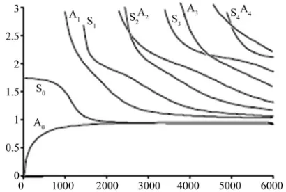
Figure 3. Dispersion curves of the phase velocity in plate

structure; Sn symmetric Lamb waves; An asymmetric Lamb

waves.

to thickness, there are present Lamb waves, Sn and An,

where n = 0, 1, 2,…, n etc. For high frequencies, and A0,

S0 Lamb waves become Rayleigh surface waves, which

lie on the upper and lower surfaces of plate structure.

4. Relation of Wave Speed versus

Frequency Thickness (Dispersion Curves)

Lamb waves are highly dispersive (phase velocity va- ries significantly with the change of frequency). How- ever, S0 wave for low values of the frequency- thickness

product shows small dispersion. In addition to finding a nontrivial solution, homogeneous

Equation (9) should have the determinant of the set of the matrix coefficients equal to zero. The determinant can be expressed as the product of four smaller determi-nants which correspond to couple coefficients (M, V), (N,

R), (T, L) (K, P).

5. Techniques of the Guided Wave

Generation at the Dispersion Curves

These equations are solved numerically allowing the determination of the possible guided waves. Any solu-tion of the characteristic equasolu-tion, defines a specific value of the wave number ξ, and so the wave velocity c. Find of the solutions leads to the relation of phase veloc-ity versus frequency or frequency thickness. These val-ues are presented in the form of dispersion curve [6].

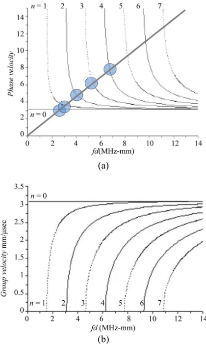
There are used two techniques for the generation of guided waves the first one is with the angular probe where the energy within the structure can be calculated through Snellit’s law. Every angle of probe defines one horizontal activation line in dispersion curves graphs (Figure 4, dot horizontal lines). By changing the fre-quency becomes possible the activation of the wave’s modes along these horizontal lines.

For Lamb waves there are constructed dispersion curves of the phase velocity (Figure 3). For low values of the frequency-thickness product, there are only two types of Lamb waves: S0, which is symmetric Lamb

wave and it is similar to longitudinal waves, and A0,

which is an asymmetric Lamb wave and it is similar to bending waves.

The second technique is realized with a comb probe where the spaces between the elements determine the slope of activation line graphs of the dispersion curve. The line is shown for a particular space, under which, by changing the frequency move along its beginning at the origin (Figure 4, continuous slope line, λ = V/f). It is For high values of the product of frequency multiplied

3 4

1 2

1 2

3 4

2 5

2

5

sin sin 0 0 0 0 0 0

cos cos 0 0 0 0 0 0

0 0 sin sin 0 0 0 0

0 0 cos cos 0 0 0 0

0 0 0 0 sin sin 0 0

0 0 0 0 sin sin 0 0

0 0 0 0 0 0 cos sin

0 0 0 0 0 0 cos cos

c d c d _M

c d c d _V

c d c d _N

c d c d R

T

c d d

L

d i d

K

dc d

P

i d d

 

 

 

 

  

   

  

   



 _{ }

 _{ }

 

  

 

 



 _ 

 

  

 

 

 _{ }

 

0

 

 

 

 

 _{ }

 

 

 

 

 

 _

possible to change the slope of line through change of the space, or by using some delay elements in the probe comb. In both techniques, maximum amplitude can be reached where the activation lines suspend the mode of the waves [7].

6. Direct Method of Testing a Planar

Structure with Guided Waves

Test consists on thickness control of a reference plate with known thickness 5.89 mm, material, by using direct method [8]. The transducer shear horizontal Emat [9] (electromagnetic transducer) with wavelengths’ λ = 12 mm, the ultrasonic device Epoch 4b. There are generated the dispersion curves for Lamb waves and shear waves for the stainless steel plate which are illustrated in Fig-ure 5 for phase velocity and group velocity versus fre-quency-thickness product. Dispersion curves for Lamb waves are shown in Figure 6.

Length of wave to shear wave is fixed through Emat magnet probe, which produces an activation line to the dispersion curves of the phase velocity versus fre-quency·thickness product, slope line is shown to Figure 5(b). The slope of activation line is determined by wave-length of the transducer.

When the activation line permeates the dispersion curve of the phase of velocity will be noted a maximum in amplitude. The corresponding frequency is called “peak frequency”.

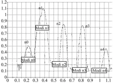
A tone-burst function generator that performs a fre-quency sweep was used to do the thickness measurement. The amplitudes of the received signals were recorded as the frequencies were swept from low to high. Figure 7 shows the results of frequency sweeping.

[image:4.595.318.528.83.433.2]

Mode n0 is not dispersive and independent of the thickness changes, so peak frequency in n0 mode of the

Figure 4. Dispersion curves and the activation lines of the guided waves.

(a)

[image:4.595.70.272.531.689.2]

(b)

Figure 5. Shear waves dispersion curves for stainless steel

plate with thickness 5.89 mm. (a) phase velocity (mm/μsec);

(b) group velocity (mm/μsec).

wave is non-changeable for the entire structure, this qual-ity makes this wave mode unsuitable to measure the thickness. n0 peak frequency is determined by the wave-length for the Emat transducer and phase velocity, which is also the shear wave velocity in the material and it, is determined by the properties of the material.

This has value because it can be used to see clearly to what kind of wave belongs a peak frequency.

As example, in an experiment by changing the fre-quency can not be predict the peak frefre-quency value for nl, n2 or other types, but we are able to understand the wave mode by comparing peak frequency with fixed frequency of n0 (Figure 7).

If this peak frequency is the first one observed after n0, it should belong to nl mode of the wave; if is the second peak frequency it belongs to n2 mode wave and so on. By recognizing the value of peak frequency and wave-length, the phase velocity can be calculated as product of peak frequency with wavelength.

E. SOTJA ET AL. 536

(a)

[image:5.595.67.277.75.396.2]

(b)

Figure 6. Lamb waves dispersion curves for stainless steel

plate with thickness 5.89 mm. (a) phase velocity (mm/μsec);

(b) group velocity (mm/μsec).

Figure 7. Frequency swep results for different mode.

can be determined by the phase velocity versus the fd to the dispersion curve as it shows Figure 5(b), by calcu-lating the value of phase velocity and known wave mode.

[image:5.595.308.538.105.191.2]

The error for the n1 is bigger than the others meas-urements. The other errors are about 1% - 1.5%. Greater dispersion of the dispersive curves brings smaller gener-ated error by determination of fd in relation to phase ve-locity. For nl mode, the curve is less dispersive at the

Table 1. Measurement results of the thickness with the di-rect method.

Mode wave

Frequency (MHz)

Real thickness (mm)

Calculated thickness (mm)

n1 0.3310 5.89 6.28

n2 0.5675 5.89 6.05

n3 0.8125 5.89 6.02

n4 1.5225 5.89 5.97

point of meeting with the line of activation, from where is explained the big error. So in high mode there is greater accuracy in measuring of the thickness.

7. Conclusions

Direct method based on achieving peak frequency of shear waves is applied in assessing the thickness of steel non-oxidizing material plate. Algorithm is built for automated drawing of dispersion curves of phase veloc-ity and group speed, the Lamb waves and shear waves. Interpretation of experimental results verifies the below results:

 the generation of the guided waves occurs only at points of dispersion curves and not in the points be-tween them;

 there is distinction between modes of the waves, in terms of improving the reception, sensitivity and power penetration. A good performance of experi-ments is achieved selecting carefully the phase veloc-ity and frequency;

 n0 mode is useful to see clearly to what kind of wave belongs a peak frequency;

 nl, n2 mode and other types mentioned above can be applied effectively in the evaluation of third parame-ter (thickness of the planar structures);

 greater dispersion of the dispersive curves brings smaller generated error by determination of f·d in re-lation to phase velocity.

8. References

[1] A. Demma, “Guided Waves: Opportunities and Limita-tions,” AIPND, International Conference, 2009. Available at http://www.ndt.net/article/aipnd2009/files/orig/ 1pdf [2] J. L. Rose, “A Baseline and Vision of Ultrasonic Guided

Wave Inspection Potential,” Transactions of the ASME,

Journal of Pressure Vessel Technology, Vol. 124, No. 3, pp 273-282, 2002. doi:10.1115/1.1491272

[3] A. Demma, D. Alleyne and B. Pavlakovic, “Uso Delle Onde Guidate per Ispezione di Tuberie Incamiciate o Interrate,” AIPND Conference 2005. Available at

[image:5.595.72.271.446.592.2]

Guided Wave Technology for Testing,” Proceedings of International Conference European NDT, 2009, pp 432- 438.

[5] T. Kundu, “Ultrasonic Non Destructive Evaluation (Chapter 4),” Cambridge University Press, Cambridge. [6] J. Rose, “Ultrasonic Waves in Solid Media,” Cambridge

University Press, Cambridge, 1999.

[7] F. Marques and A. Demma, “Ultrasonic Guided Waves Evaluation of Trials for Pipeline Inspection,” 17th World

Conference on Non Destructive Testing, 25-28 October 2008, Shanghai. Available at

http://www.ndt.net/article/wcndt2008/papers/96.pdf [8] Y. Cho, “Guided Wave Monitoring of thickness Variation

for Thin Film Materials,”Materials Evaluation, Vol. 61, No. 3, 2003, pp. 418-422.