Economics Working Paper Series
2017/014
Inference in Nonparametric Series Estimation with
Data-Dependent Undersmoothing
Byunghoon Kang
The Department of Economics Lancaster University Management School
Lancaster LA1 4YX UK
© Authors
All rights reserved. Short sections of text, not to exceed two paragraphs, may be quoted without explicit permission,
provided that full acknowledgement is given.
Inference in Nonparametric Series Estimation with
Data-Dependent Undersmoothing
Byunghoon Kang
∗Department of Economics, Lancaster University
First version December 9, 2014; Revised May 16, 2017
Abstract
Existing asymptotic theory for inference in nonparametric series estimation
typ-ically imposes an undersmoothing condition that the number of series terms is
suf-ficiently large to make bias asymptotically negligible. However, there is no formally
justified data-dependent method for this in practice. This paper constructs inference
methods for nonparametric series regression models and introduces tests based on the
infimum of t-statistics over different series terms. First, I provide an empirical process
theory for the t-statistics indexed by the number of series terms. Using this result,
I show that test based on the infimum of the t-statistics and its asymptotic critical
value controls asymptotic size with undersmoothing condition. Using this test, we can
construct a valid confidence interval (CI) by test statistic inversion that has correct
asymptotic coverage probability. Allowing asymptotic bias without the
undersmooth-ing condition, I show that CI based on the infimum of the t-statistics bounds coverage
distortions. In an illustrative example, nonparametric estimation of wage elasticity of
the expected labor supply from Blomquist and Newey (2002), proposed CI is close to
or tighter than those based on the standard CI with the possible ad hoc choice of series
terms.
Keywords: Nonparametric series regression, Pointwise confidence interval,
Smooth-ing parameter choice, Specification search, UndersmoothSmooth-ing.
JEL classification: C12, C14.
∗This paper is a revised version of my first chapter in the Ph.D. thesis at UW-Madison. I am deeply
indebted to Bruce Hansen for his continuous guidance and suggestions. I am also grateful to Jack Porter, Xiaoxia Shi and Joachim Freyberger for thoughtful discussions. Thanks to Michal Koles´ar, Denis Chetverikov, Yixiao Sun, Andres Santos, Patrik Guggenberger, Federico Bugni, Joris Pinkse, Liangjun Su, and Myung Hwan Seo for helpful conversations and criticism. I acknowledge support by Kwanjeong Educational Foundation Graduate Research Fellowship and Leon Mears Dissertation Fellowship from UW-Madison. All errors are my own. Email: [email protected], Homepage:
1
Introduction
I consider the following nonparametric regression model;
yi =g0(xi) +εi,
E(εi|xi) = 0
(1.1)
where {yi, xi}ni=1 is i.i.d. with scalar response variable yi, vector of covariates xi ∈ Rdx, and
g0(x) = E(yi|xi =x) is the conditional mean function. Examples falling into the model (1.1)
include nonparametric estimation of the Mincer equation, gasoline demand, and labor
sup-ply function (see, among many others, Heckman, Lochner and Todd (2006), Hausman and
Newey (1995), Blomquist and Newey (2002), Blundell and MaCurdy (1999), and references
therein). Addressing potential misspecification of the parametric model, nonparametric
se-ries methods have several advantages, as they can easily impose shape restrictions such as additive separability or concavity, and implementation is easy because the estimation method
is least squares. However, implementation in practice requires a choice of the number of
se-ries terms,K. Estimation and inference may largely depend on its choice in finite samples.
Moreover, required K may vary with different data sets to accommodate the smoothness of
unknown function and different sample sizes, as well as whether the goal is estimation or
inference.
Existing theory for the asymptotic normality and valid inference imposes so-called
under-smoothing (i.e.,overfitting) condition that is a faster rate ofK than the mean-squared error
(MSE) optimal convergence rates to make bias asymptotically negligible relative to standard deviation. The undersmoothing condition has been imposed, particularly for valid inference,
in many nonparametric series methods both in theory and in practice, as there is no theory
for bias-corrections available to date. Ignoring asymptotic bias with the undersmoothing
assumption, one can apply the conventional confidence interval (CI) using the standard
nor-mal critical value with estimates and standard errors based on some choice of “sufficiently
large” K (larger than MSE optimal K). However, the asymptotic theory does not provide
specific guidelines for choosing a “large” number of series terms to make bias small in
prac-tice. With given sample sizesn, some possibly ad hoc methods in practice selectKb =Ke·nγ
with some pre-selected Ke and a specific rate of γ that satisfies the undersmoothing level,
which is generally unknown. However, there is no formally justified data-dependent method
to choose K that gives the desired level of undersmoothing in series regression literature.
Due to these unsatisfactory results for the inference procedure both in theory and
prac-tice, a specification search seems necessary, i.e., search over different series termsK ∈[K,K¯].
regres-sion, or try a different number of knots in regression spline to see how the estimate and
standard error change. Moreover, some data-dependent selection rules that are valid for
estimation (such as cross-validation) and some rule-of-thumb methods that are suggested
for inference, also require evaluating estimates with different Ks. If researchers evaluate
different specifications with a different number of series terms and select one specification as
a baseline model, it is not clear how this randomness affects the standard inference.
In this paper, I construct inference methods in nonparametric series regression given the
range of different series terms. I consider the testing problem for a regression function at a
point and introduce tests based oninfimum of the studentized t-statistics over different series
terms. To describe intuition heuristically, we may decompose infimum t-statistic as follows
inf
K |Tn(K)| ≈infK |N(0,1) +
Bias(K)
SE(K) |
where Tn(K), Bias(K), SE(K) denote t-statistic, bias and standard error of the series
esti-mator usingK terms, respectively. The test based on infimum t-statistics and searching for
small t-statistics have a similar motivation to the one on which the undersmoothing
condi-tion is theoretically based: using faster rates ofK than the optimal MSE rate (using “large”
K that has a small bias and large variance) so that makes the second term, Bias(K)SE(K) , small.
Many papers in nonparametric series estimation literature typically suggested to increase
the number of series terms and include additional terms than those cross-validation chooses
for inference (for example, see Newey (2013), Newey, Powell, and Vella (1999)). Although I do not consider data-dependent methods that satisfy desired undersmoothing rates in this
paper, I formally justify this conventional wisdom by introducing the infimum test
statis-tic and provide an inference method based on its asymptostatis-tic distribution as an alternative
data-dependent undersmoothing.
For this, I first provide an empirical process theory for the t-statistics, which I shall call
t-statistic process, indexed by the number of series terms. The main contribution of this
paper is to derive a uniform asymptotic distribution theory for the entire sequences of
t-statistics over a range ofK. Existing asymptotic normality of the t-statistic in the literature
holds under a deterministic sequence of K → ∞ as the sample size increases. I impose an assumption on the set of deterministic sequences Kn where the number of series terms
K ∈ Kn can be indexed by continuous parameter π, a ‘fraction’ of the largest series terms
¯
K, and this is important for our purpose to show the weak convergence of the empirical
process.
Using this result, I show that test based on the infimum of the t-statistics and its
under-smoothing condition for allKs in a set. Allowing asymptotic bias without the
undersmooth-ing condition, I also analyze the effect of bias on the asymptotic size of the test. Even
allowing the asymptotic bias, the test based on the infimum t-statistic bound the size
dis-tortions, in the sense that the asymptotic size is bounded above by the asymptotic size of a
test with a t-statistic that has the smallest bias. The infimum t-statistic is less sensitive to
the asymptotic bias: it naturally excludes small K with large bias and selects among some
large Ks under the null.
I also construct a valid pointwise confidence interval for the conditional mean function
that has nominal asymptotic coverage probability by test statistic inversion. The proposed
CI based on infimum test statistic can be easily constructed using estimates and standard errors for the set of Ks. It is obtained as the union of all CIs by replacing the standard
normal critical value with the critical value from the asymptotic distribution of the infimum
t-statistic. We can approximate the asymptotic critical value using a simple Monte Carlo
or weighted bootstrap method. Similar to the asymptotic size results, I show that proposed
CI bounds the coverage distortions even when asymptotic bias exists. I also find that our
proposed CI performs well in Monte Carlo experiments; coverage probability of the CI based
on the infimum t-statistic is close to the nominal level in various simulation setups. As an
illustrative example, I revisit nonparametric estimation of wage elasticity of the expected
labor supply, as in Blomquist and Newey (2002). Given the table in Blomquist and Newey (2002), the proposed CI is tighter than the standard CI with the largest number of series
terms as well as close to the standard CI with some “large” K.
This paper also provides a valid CI after selecting the number of series terms. By
ad-justing the conventional normal critical value to the critical value from supremum of the
t-statistics over all series terms, we can adjust uncertainty due to the choice of series terms.
This paper gives a valid post-selection CI that has a correct coverage with any choice of Kb
among some ranges. By enlarging the CI with critical values larger than the normal critical
value, this post-selection CI can accommodate bias, although it does not explicitly deal with
bias problems. We expect this lead to a tighter CI than those based on the Bonferroni-type critical value, as I incorporate the dependence structure of the t-statistics from our
asymptotic distribution theory.
I also investigate inference methods in partially linear model setup. Focusing on the
common parametric part, choice problems also occur for the number of approximating terms
or the number of covariates in estimating the nonparametric part. Unlike the nonparametric
object of interest that has a slower convergence than n1/2 rate (e.g., regression function or
regression derivative), t-statistics for the parametric object of interest are asymptotically
fully account for the dependency of the t-statistics with the different sequences of Ks in the
partially linear model setup, this requires a different approximation theory than standard
first order approximation results. Using the recent results of Cattaneo, Jansson, and Newey
(2015a), I develop a joint asymptotic distribution of the studentized t-statistics over a
dif-ferent number of series terms. By focusing on the faster rate of K that grows as fast as the
sample sizen and using larger variance than the standard variance formula, we can account
for the dependency of t-statistics with different Ks. In this setup, I also propose methods
to construct CIs that are similar to the nonparametric regression setup and provide their
asymptotic coverage properties.
1.1
Related literature
The literature on nonparametric series estimation is vast, but data-dependent series term se-lection and its impact on estimation or inference are comparatively less developed. Perhaps
the most widely used data-dependent rule in practice is cross-validation. Asymptotic
opti-mality results have been developed (see, for example, Li (1987), Andrews (1991b), Hansen
(2015)) in terms of asymptotic equivalence between integrated mean squared error (IMSE)
of the nonparametric estimator with Kbcv selected by minimizing the cross-validation
crite-rion and IMSE of the infeasible optimal estimator. However, there are two problems with
cross-validation selected Kbcv for the valid inference. First, it is asymptotically equivalent to
selecting K to minimize IMSE, and thus it does not satisfy the undersmoothing condition
needed for asymptotic normality without bias terms. Therefore, a t-statistic based on Kbcv will be asymptotically invalid for inference. Second, Kbcv selected by cross-validation will
itself be random and not deterministic. Thus, it is not clear whether the t-statistic based
onKbcv has a standard asymptotic normal distribution which is derived from a deterministic
sequence of K.
Novel recent papers by Horowitz (2014), Chen and Christensen (2015a) develop the
state-of-the-art data-dependent methods in the nonparametric instrumental variables (NPIV)
es-timation (see also other references therein). They develop data-driven methods for choosing
sieve dimension in that resulting NPIV estimators attain the optimal sup-norm or L2 norm
rates adaptive to the unknown smoothness of g0(x). In this paper, we focus on the inference
rather than estimation with the similar issues arise from using cross-validation.
Moreover, this paper is also closely related to the previous methods that conceptually
require increasing K until t-statistic is “small enough”. For example, among many others,
Newey (2013) suggested increasingKuntil standard errors are large relative to small changes
those cross-validation chooses, and Horowitz and Lee (2012) suggested increasing K until
the integrated variance suddenly increases and then adding an additional term. They discuss
these methods work well in practice and simulation. Using similar ideas, I provide formal
inference methods based on asymptotic distribution results of the infimum test statistic with
appropriate critical values smaller than the standard normal critical values.
Several important papers have investigated the asymptotic properties of series (and
sieves) estimators, including papers by Andrews (1991a), Eastwood and Gallant (1991),
Newey (1997), Chen and Shen (1998), Huang (2003a), Chen (2007), Chen and Liao (2014),
Chen, Liao, and Sun (2014), Belloni, Chernozhukov, Chetverikov, and Kato (2015), and
Chen and Christensen (2015b), among many others. Under i.i.d. or weakly dependent data, they focused on Sup/L2-norm convergence rates, asymptotic normality of series estimators,
and pointwise/uniform inference on linear/nonlinear functionals under a deterministic
se-quence of K. This paper extends the asymptotic normality of the t-statistic under a single
sequence of K to the uniform central limit theorem of the t-statistic for the sequences of K
over a set, and focuses on a pointwise inference on g0(x), which is an irregular (i.e., slower
than n1/2 rate) and linear functional, under i.i.d. data.
For the kernel-based density or regression estimation, the data-dependent bandwidth
selection problem is well known. Several rule-of-thumb methods and plug-in optimal
band-widths have been proposed (see H¨ardle and Linton (1994), Li and Racine (2007) for ref-erences). A recent paper by Calonico, Cattaneo and Farrell (2015) compared higher-order
coverage properties of undersmoothing and explicit bias-corrections and derived coverage
op-timal bandwidth choices in kernel estimation. See also Hall and Horowitz (2013), Schennach
(2015) and references therein for various recent work on related bias issues and
nonparamet-ric inference for the kernel estimator. Unlike the kernel-based methods, little is known about
the statistical properties of data-dependent selection rules (e.g., rates of Kbcv) and
asymp-totic distribution with data-dependent methods in series estimation. In general, the main
technical difficulty arises from the lack of an explicit asymptotic bias formula for the series
estimator (see Zhou, Shen, and Wolfe (1998) and Huang (2003b) for exceptions with some specific sieves). Thus, it is difficult to derive an asymptotic theory for the bias-correction,
or some plug-in formulas compare with kernel estimation.
An important recent paper that is concurrent with this paper, Armstrong and Koles´ar
(2015) considered inference methods in kernel estimation with bandwidth snooping.
Fo-cusing on the supremum of the t-statistics over the bandwidths, they developed confidence
intervals that are uniform in bandwidths. Considering supremum statistic is motivated by
the sensitivity analysis as a correction for the multiple testing problems. Moreover,
has been used to achieve adaptive inference procedures when smoothness of the function is
unknown (See Horowitz and Spokoiny (2001), and also Armstrong (2015)). See Appendix C
for the similar coverage results (uniform in series terms) as in Armstrong and Koles´ar (2015).
The main focus of this paper is to analyze the undersmoothing assumption with their effect
on the size of the tests and to develop tests which can control size distortions even allowing
large asymptotic bias, which can be crucial in series estimation context.1
The outline of the paper is as follows. I first introduce basic nonparametric series
regres-sion setup in Section 2. In Section 3, I provide an empirical process theory for the t-statistic
sequences over a set. Section 4 introduces infimum of the t-statistic and describes the
asymp-totic null distributions of the test statistic. Then, I provide the asympasymp-totic size results of the test and implementation procedure for the critical value. Section 5 introduces CIs based
on the infimum test statistic and provides their coverage properties. Section 6 analyzes valid
post model selection inference in this setup. Section 7 extends our inference methods to the
partially linear model setup. Section 8 includes Monte Carlo experiments in various setups.
Section 9 illustrates proposed inference methods using the nonparametric estimation of wage
elasticity of the expected labor supply, as in Blomquist and Newey (2002), then Section 10
concludes. Appendix A and B include all proofs, figures, and tables. Appendix C discuss
inference procedures based on the supremum of the t-statistics.
1.2
Notation
I introduce some notation will be used in the following sections. I use ||A||=ptr(A0A) for
the Euclidean norm. Let λmin(A), λmax(A) denote the minimum and maximum eigenvalues
of a symmetric matrix A, respectively. op(·) and Op(·) denote the usual stochastic order
symbols, convergence in probability and bounded in probability. −→d denotes convergence
in distribution and ⇒ denotes weak convergence. I use the notation a ∧b = min{a, b},
a∨b= max{a, b}, and denotebac as the largest integer less than the real numbera. For two
sequences of positive real numbers an and bn, an .bn denotesan ≤cbn for all n sufficiently
large with some constant c > 0 that is independent of n. an bn denotes an . bn and
bn . an. For a given random variable {Xi} and 1 ≤ p < ∞, Lp(X) is the space of all
Lp norm bounded functions with ||f||Lp = [E||f(Xi)||p]1/p and `∞(X) denotes the space of all bounded functions under sup-norm, ||f||∞ = supx∈X|f(x)| for the bounded real-valued
functions f on the support X. Let also R+ = {x ∈ R : x ≥ 0}, R+,∞ = R+ ∪ {+∞},
R[+∞]=R∪ {+∞} and R[±∞] =R∪ {+∞} ∪ {−∞}.
2
Model framework and estimation
I first introduce the nonparametric series regression setup in the model (1.1). Given a random
sample{yi, xi}ni=1, we are interested in the conditional meang0(x) = E(yi|xi =x) at a point
x∈ X ⊂Rdx. All the results derived in this paper are the pointwise inference in xand I will
omit the dependence on x if there is no confusion.
We consider the sequence of approximating model indexed by the number of series terms
K ≡ K(n). Let bgK(x) be an estimator of g0(x) using the first K vectors of approximating
functions PK(x) = (p1(x),· · ·, pK(x))0 from basis functionsp(x) = (p1(x), p2(x),· · ·)0.
Stan-dard examples for the basis functions are power series, Fourier series, orthogonal polynomials
(e.g., Hermite polynomials), or splines with evenly sequentially spaced knots.
Series estimator bgK(x) is then obtained by standard least square (LS) estimation of yi
on regressors PKi
b
gK(x) =PK(x)0βbK, βbK = (PK 0
PK)−1PK0Y (2.1)
where PKi ≡ PK(xi) = (p1(xi), p2(xi),· · ·, pK(xi))0, PK = [PK1,· · ·, PKn]0, Y = (y1,· · ·yn)0.
b
gK(x) is an estimator of the best linear L2 approximation for g0(x), i.e., PK(x)0βK where
βK is defined as the best linear projection coefficients βK ≡ (E[PKiPKi0 ])
−1E[P
Kiyi]. Define
the approximation error using K series terms as rK(x) = g0(x)− PK(x)0βK for x ∈ X.
Also define rKi ≡ rK(xi), pi ≡ p(xi) = (p1i, p2i,· · ·,)0. We can write the model using K
approximating terms as the following projection model
yi =PKi0 βK+εKi, E[PKiεKi] = 0 (2.2)
where εKi ≡rKi+εi.
For simplicity of notation, I define the true regression function at a point as θ0 ≡g0(x).
LetθbK ≡ b
gK(x) and θK ≡PK(x)0βK. Define the series variance
VK ≡VK(x) =PK(x)0QK−1ΩKQ−K1PK(x),
QK =E(PKiPKi0 ), ΩK =E(PKiPKi0 ε 2
i)
(2.3)
whereQ−K1ΩKQ−K1 is the conventional asymptotic variance formula for the LS estimator βbK.
We use notion of testing setup and consider two-sided testing for θ
The studentized t-statistic forH0 is
Tn(K, θ0)≡ √
n(bgK(x)−g0(x))
VK1/2 =
√
n(bθK−θ0)
VK1/2 . (2.5)
Under standard regularity conditions (will be discussed in Section 3) including an
under-smoothing rate for deterministic sequence K → ∞ as n → ∞, the asymptotic distribution
of the t-statistic is well known
Tn(K, θ0) d
−→N(0,1).
See, for example, Andrews (1991a), Newey (1997), Belloni et al. (2015), Chen and
Chris-tensen (2015b) among many others. In the next section, I formally develop an asymptotic
distribution theory of Tn(K, θ0) over a set Kn.
3
Asymptotic distribution
3.1
Weak convergence of t-statistic process
In this section, I provide an asymptotic theory of the joint t-statistics over a set. First,
I introduce following set Kn to construct empirical process theory of the t-statistics over
K ∈ Kn that can be indexed by the continuous and fixed parameter π, which is a ‘fraction’
of the largest series term ¯K.
Assumption 3.1. (Set of number of series terms) Let Kn as
Kn={K :K ∈[πK,¯ K¯]}
where K =πK¯ with a fixed constant π∈Π = [π,1], π >0, and K¯ ≡K¯(n)→ ∞ asn → ∞.
Assumption 3.1 considers a range of the number of series terms and considers an infinite
sequence of approximations indexed by π ∈ Π. Note that Kn is indexed by sample size n
as I will impose rate conditions for the largest series term ¯K in the next Assumption 3.2.
Together with the Assumption 3.2 below, set Kn in Assumption 3.1 considers the sequence
of models that has the same rate of K, i.e., K K0 for any K, K0 ∈ Kn. Note that
standard inference methods in nonparametric regression setup typically consider a singleton
Next, define the following empirical process, Tn∗(π, θ), as
Tn∗(π, θ)≡Tn(bπK¯c, θ), π∈Π, (3.1)
where Tn(K, θ) is defined in (2.5), i.e., Tn∗(π, θ) is a t-statistic evaluated at the parameter θ
using bπK¯c number of series terms. Note that Tn∗(π, θ) is indexed by π ∈ Π and is a step
function of π.
Also, I impose mild regularity conditions that are standard in nonparametric series
re-gression literature and are satisfied by well-known basis functions. For each K ∈ Kn,
de-fine ζK ≡ supx∈X||PK(x)|| as the largest normalized length of the regressor vector and
λK ≡(λmin(QK))−1/2 for K×K design matrix QK =E(PKiPKi0 ).
Assumption 3.2. (Regularity conditions)
(i) {yi, xi}ni=1 are i.i.d random variables satisfying the model (1.1).
(ii) supx∈XE(ε2i|xi =x)<∞, infx∈XE(ε2i|xi =x)>0, andsupx∈XE(ε2i{|εi|> c(n)}|xi =
x)→0 for any sequence c(n)→ ∞ as n→ ∞.
(iii) For each K ∈ Kn, as K → ∞, there exists η and cK, `K such that
sup
x∈X
|g0(x)−PK(x)0η| ≤`KcK, E[(g0(xi)−PK(xi)0η)2]1/2 ≤cK.
(iv) supK∈KnλK .1.
(v) supK∈KnζK
p
(logK)/n(1 +√K`KcK) +`KcK →0 as n → ∞.
I closely follow assumptions in recent papers by Belloni et al. (2015), Chen and Chris-tensen (2015b) and impose rate conditions ofK uniformly overKn. Other standard regularity
conditions in the literature (e.g., Newey (1997)) can also be used here. Assumption 3.2(ii)
imposes moment conditions and standard uniform integrability conditions. ζK, cK, `K in
As-sumption 3.2(iii)-(v) are satisfied with various basis functions. For example, if the supportX
is a cartesian product of compact connected intervals (e.g. X = [0,1]dx) and the probability
density of xi is bounded below zero, then ζK . K for power series and other orthogonal
polynomial series, and ζK . √
K for regression splines, Fourier series, and wavelet series.
cK and `K in Assumption 3.2(iii) vary with the different basis and can be replaced by series
specific bounds. For example, if g0(x) belongs to the H¨older space of smoothness p, then
of orders0 (see Newey (1997), Chen (2007), Belloni et al. (2015), and Chen and Christensen
(2015b) for more discussions on cK, `K, ζK with various sieve bases).
When the probability density function of xi is uniformly bounded above and bounded
away from zero over the compact support X and orthonormal basis is used, then λK . 1
(see, for example, Proposition 2.1 in Belloni et al. (2015) and Remark 2.2 in Chen and
Christensen (2015b)). The rate conditions in Assumption 3.2(v) can be replaced by the
specific bounds of ζK, cK, `K. For example, for the power series, Assumption 3.2(v) reduced
to supK∈Kn
p
K2(logK)/n(1 + K3/2−p/dx) + K1−p/dx = pK¯2(log ¯K)/n(1 + ¯K3/2−p/dx) + ¯
K1−p/dx →0 under Assumption 3.1.
For notational simplicity, it is convenient to define Pπ(x) ≡ PbKπ¯ c(x), Pπi ≡ Pπ(xi) =
PbKπ¯ ci and rπ ≡rπ(x) =rbKπ¯ c(x) under Assumption 3.1. The series variance can be defined
as Vπ ≡ Vπ(x) = ||Ω 1/2
π Q−π1Pπ(x)||2, where Ωπ = E(PπiPπi0 ε2i), Qπ = E(PπiPπi0 ). Under
Assumptions 3.1 and 3.2, the t-statistic process under H0 can be decomposed as follows
Tn∗(π, θ0) =
1
√
n
n
X
i=1
Pπ(x)0Pπiεi
Vπ1/2
−√nVπ−1/2rπ +op(1), π∈Π (3.2)
where the first term converges to a standard normal distribution for any π ∈ Π, and the
second term does not necessarily converge to 0 even with large sample sizes due to
approxima-tion errors. We want to show weak convergence of the empirical process{Tn∗(π, θ0) :π ∈Π}.
This empirical process has a covariance kernel
Σn(π1, π2)≡
Pπ1(x)
0E(P
π1iP
0
π2iε
2
i)Pπ2(x)
Vπ1/21 V
1/2
π2
, π1, π2 ∈Π. (3.3)
We expect that the limiting Gaussian process has a covariance function as a limit of the
sequence of covariance functions Σn(π1, π2), which is assumed to exist by the following
as-sumption. I also impose rate restrictions on series variances.
Assumption 3.3.
(i) Σ(π1, π2) = limn→∞Σn(π1, π2) exists and Σ(π1, π2)<1 for any π1, π2 ∈Π.
(ii) limn→∞Vπ1/2( ¯Kπ)−η =cuniformly in π ∈Π for some constants c, η >0.
Assumption 3.3(i) guarantees well-defined covariance function for the tight Gaussian
process in`∞(Π) and a positive definite variance-covariance matrix for its finite dimensional
limit distributions. Assumption 3.3(ii) may be stronger than necessary, but required to
variance is increasing in K at some rates uniformly in K ∈ Kn under Assumption 3.1, i.e.,
limn→∞V
1/2
K K
−η =c. This assumption holds with η= 1/2 when we consider a point x∈ X
where VK1/2 ∝ K1/2. Moreover, Assumption 3.3(ii) is a sufficient condition for Assumption
3.3(i) under homoskedasticity. Under conditional homoskedasticity, E(ε2
i|xi =x) = σ2, the
limit of the covariance kernel Σ(π1, π2) reduces to the simple form
Σ(π1, π2) = lim
n→∞
Vπ1/21∧π2
Vπ1/21∨π2
(3.4)
for anyπ1, π2 ∈Π, i.e., the covariance kernel is the limit of the ratio of standard deviations. If
we further assume Assumption 3.3(ii), then Σ(π1, π2) = (ππ11∨∧ππ22)
η. Withη= 1, this coincides
with the covariance kernel of a scaled Brownian motion process Z(π)/√π, π ∈Π.
Next, I define the asymptotic bias for the sequence of models indexed by π as the limit of the second term in (3.2)
ν(π)≡ lim
n→∞−
√
nVπ−1/2rπ. (3.5)
Under the following undersmoothing condition, ν(π) = 0 for all π ∈ Π. To assess
the effect of bias on inference, we will consider a distinction between results imposing the
undersmoothing condition or not.
Assumption 3.4. (Undersmoothing) sup
K∈Kn
|√nVK−1/2`KcK| →0 as n→ ∞.
When we use explicit bounds `KcK .K−p/dx for spline or wavelet series, Assumption 3.4
reduces to sup
K∈Kn
√
nVK−1/2K−p/dx = o(1). When we further consider V1/2
K ∝ K
1/2,
Assump-tion 3.1 and 3.4 together imply that AssumpAssump-tion 3.4 is provided by √nK¯1/2−p/dx → 0 for power series.
Next theorem is our first main result which provides uniform central limit theorem of the
t-statistic process for nonparametric LS series estimation.
Theorem 3.1. Under Assumptions 3.1, 3.2, 3.3 and supπ|ν(π)|<∞,
Tn∗(π, θ0)⇒T(π) +ν(π), π ∈Π, (3.6)
whereT(π)is a mean zero Gaussian process on`∞(Π)with covariance kernelE(T(π1)T(π2)) =
satisfied, then
Tn∗(π, θ0)⇒T(π), π ∈Π. (3.7)
Theorem 3.1 provides weak convergence of the t-statistic processTn∗(π, θ0), π∈Π. This is
an asymptotic theory for the entire sequence of t-statisticsTn(K, θ0), K ∈ Kn. The t-statistic
process converges weakly to a mean zero Gaussian process T(π) plus the asymptotic bias
ν(π). Proof of Theorem 3.1 needs to verify a uniform-entropy condition and apply empirical
process theory in van der Vaart and Wellner (1996, Theorem 2.11.22).
Remark 3.1 (Rate conditions). Note that the asymptotic bias |ν(π)| = 0 if ¯K increases faster than the optimal MSE rate (undersmoothing). 0 <|ν(π)| <∞ if ¯K increases at the
optimal MSE rate, and|ν(π)|= +∞if ¯K increases slower than the optimal MSE rate
(over-smoothing). Theorem 3.1 does not allow oversmoothing rates as we require supπ|ν(π)|<∞.
Assumption 3.1 does not consider different rates ofK satisfying asymptotic normality of
se-ries estimators, however, these are the class of sequences to be able to provide uniform
central limit theorem of the t-statistic process. As studentized t-statistic is normalized by the standard deviation VK1/2 which may increase differently with different rates of K, two
t-statistics with different rates of K can be asymptotically independent, thus hard to
in-corporate dependency (see discussions in Section 3.2 with alternative Kn allowing different
rates of K).
Remark 3.2 (Other functionals). Here, I focus on the leading example, where θ0 = g0(x)
for some fixed point x ∈ X, but I may consider other linear functionals θ0 = a(g0(·)), such
as the regression derivatesa(g0(x)) = dxdg0(x). All the results in this paper can be applied to
irregular (slower than n1/2 rate) linear functionals with estimators
b
θ =a(bgK(x)) =aK(x)0βbK
and appropriate transformation of basisaK(x) = (a(p1(x),· · ·, a(pK(x)))0. While verification
of previous results for regular (n1/2 rate) functionals, such as integrals and weighted average
derivative, is beyond the scope of this paper, I examine similar results for the partially linear
model setup in Section 7.
3.2
Asymptotic normality with different rates
Next, we provide different asymptotic distribution of the sequence of t-statistics with an alternative set Kn constructed to allow different rates of Ks. A following alternative set
assumption allows for optimal mean squared error rates ofK as well as oversmoothing rates
which increase slower than the optimal MSE rates.
Kn = {K = K1,· · ·, Km,· · ·,K¯ = KM} where Km ≡ bτ nφmc for constant τ > 0,
0 < φ1 < φ2 < · · · < φM, and fixed M. Define asymptotic bias for the sequence
of models as ν(m) ≡ − lim
n→∞
√
nVK−1/2
m rKm. Assume that the largest model K¯ satisfies
√
nVK−¯1/2`K¯cK¯ →0 as n → ∞.
Assumption 3.5 can consider rates of K from oversmoothing (|ν(m)| = +∞) to
under-smoothing (|ν(m)| = 0) with different φm. Here, K can increase slower than the optimal
MSE rates and ¯K satisfies undersmoothing rates. Assumption 3.5 considers a broader range
of Ks than the Assumption 3.1 as alternative set allows slower than optimal MSE rates.
Together with Assumption 3.2, there exist explicit rate restrictions on φm uniformly over m
to guarantee an asymptotic normality of each single t-statistic. Undersmoothing assumption
for the ¯K, i.e. ν(M) = 0, is a modeling device considering a broad range of K and large
enough ¯K so that satisfy undersmoothing.
Under Assumption 3.5, joint t-statistics do not converge in distribution to a bounded
random vector if any of the elements|ν(m)|= +∞with oversmoothing sequences. Ifν(m) =
±∞ for some m, then it can be shown that corresponding t-statistic Tn(Km, θ0) diverges in
probability to ±∞. This matters when we obtain the asymptotic distribution of the test
statistic that is some continuous transformation of the joint t-statistics because continuous
mapping theorem cannot be directly applied. This technical difficulty does not arise when
we consider t-statistics centered at the true conditional mean function (θ0) with relative bias
(rKm) and standard error (
p
VKm/n): joint t-statistics converge in distribution to a mean
zero normal random vector. However, allowing |ν(m)| = +∞ is important for our analysis to consider asymptotic bias and undersmoothing (and oversmoothing) condition with their
effects on inference.
To obtain the asymptotic distribution under supm|ν(m)|= +∞, we provide formal proofs
which combine arguments in inference on CIs for the parameters in moment inequality
liter-ature as in Andrews and Guggenberger (2009). For this, we define the continuous function
on the extended real space as follows; S : A→ B is continuous at t ∈ A if t0 → t for t ∈ A
implies S(t0)→S(t) for any set A.
Theorem 3.2. Under Assumptions 3.2 and 3.5, following holds for any continuous function S(t) at all t ∈RM−1
[±∞]×R,
S(Tn(θ0)) d
−→S(Z+ν)
where Tn(θ) = (Tn(K1, θ),· · ·, Tn(KM, θ))0, Z = (Z1,· · ·, ZM)0 ∼ N(0,Σ), ν = (ν(1),· · ·,
with Σjl = limn→∞Σjl,n, and Σjl,n =
PKj(x)0E(PKj iPKli0 ε2
i)PKl(x)
VKj1/2VKl1/2 . If ν(m) = ±∞, then the
corresponding element of Z +ν equals ±∞.
Note that we do not require either Assumption 3.4 (undersmoothing) or supm|ν(m)|<
∞ in Theorem 3.2. Variance-covariance matrix Σ is similarly defined as in Theorem 3.1.
Moreover, if VK1/2 Kη at some point x with η > 0, then for any j < l, Σ
jl,n ≤ C
VKj1/2
VKl1/2 for
some constant C > 0 by Assumption 3.2(ii) and the upper bound converges to 0 as n →0
by Assumption 3.5, thus Σjl,n →0 and Σ =IM.
Remark 3.3 (Rate conditions (continued)). Note that Assumption 3.5 only considers finite sequences, i.e.,|Kn|=M. Assumption 3.5 is useful to consider the effect of bias on inference
problems allowing a broader range of K including oversmoothing rates (see Section 4 for
formal results). On the other hand, Assumption 3.1 considers sequences of K with the
same rates which only differ in constant π. Thus, Theorem 3.1 gives the joint asymptotic distribution of t-statistics that has either zero bias for allK ∈ Kn or non-zero bounded bias
for all K ∈ Kn.
4
Test statistic
In this section, I introduce an infimum test statistic and analyze its asymptotic null
distri-bution based on Theorem 3.1 and 3.2. Then, I provide an asymptotic size result of the tests,
and methods to obtain critical values for inference procedures. I consider following test statistic
InfTn(θ)≡ inf
K∈Kn
|Tn(bKc, θ)|, (4.1)
where either Assumption 3.1 or Assumption 3.5 can be used for Kn. Note that InfTn(θ) =
infπ∈Π|Tn∗(π, θ)| under Assumption 3.1 and InfTn(θ) = infm=1,···,M|Tn(Km, θ)| under
As-sumption 3.5.
As I denoted in the introduction, there are several reasons to consider InfTn(θ) in the
series regression context. First of all, small t-statistic centered at the true θ0 corresponds
to the approximation with a certain choice of series terms that has a small bias and large
variance, which is good for inference similar to what undersmoothing assumption does by eliminating asymptotic bias, theoretically. Moreover, this is also closely related to some
rule-of-thumb methods suggested by several papers to choose undersmoothed K (see, for
4.1
Asymptotic distribution of the test statistic
Asymptotic null limiting distribution of the infimum test statistic follows immediately from
Theorem 3.1 and 3.2.
Corollary 4.1. 1. Under Assumptions 3.1, 3.2, 3.3 andsupπ|ν(π)|<∞, InfTn(θ0) d −→
infπ∈[π,1]|T(π) +ν(π)|, whereT(π) is the mean zero Gaussian process defined in
Theo-rem 3.1. In addition, if Assumption 3.4 holds, thenInfTn(θ0) d
−→ξinf ≡infπ∈[π,1]|T(π)|.
2. Under Assumptions 3.2 and 3.5, InfTn(θ0) d
−→ infm=1,···,M|Zm+ν(m)|, where Zm is
an element of M×1 normal vector Z ∼N(0,Σ) and ν= (ν(1),· · ·, ν(M))0 is defined
in Theorem 3.2.
Corollary 4.1.1 derives the asymptotic null limiting distribution of InfTn(θ) underKnwith
same rates of K (Assumption 3.1) and Corollary 4.1.2 provides the asymptotic distribution
under alternative Kn with different rates of K (Assumption 3.5).
Whether some asymptotic bias |ν(m)|are unbounded or not, Corollary 4.1.2 shows that InfTn(θ0) converge in distribution to the bounded random variable. Under the null H0,
InfTn(θ) exclude all small Ks corresponding to oversmoothing rates (where the bias is of
larger order than the standard error) and select among large Ks with optimal MSE rates
and undersmoothing rates (where the bias is of smaller order), asymptotically. Using this
Corollary, I discuss the effect of asymptotic bias on the inference in Section 4.2 (for the size
results) and Section 5 (for the coverage results).
4.2
Asymptotic size
I start by defining critical value cinf
1−α as (1−α) quantile of the asymptotic null distribution
ξinf = infπ∈[π,1]|T(π)| in Corollary 4.1.1, i.e., solves
P( inf
π∈[π,1]|T(π)|> c inf
1−α) =α (4.2)
for 0< α <1/2.2
The asymptotic null distribution, ξinf, can be completely defined by covariance kernel of
the limiting Gaussian process T(π) in Theorem 3.1. In the special case where Assumption
3.3(ii) holds with η = 1 under homoskedasticity (as discussed below the equation (3.4)),
2Without imposing the undersmoothing assumption, asymptotic distribution of InfT
n(θ0) in Corollary
4.1.1 also depend on asymptotic bias ν(π) as well. If ν(π) can be replaced by some estimates bν(π), then the critical value from infπ∈Π|T(π) +bν(π)|can be used. We do not pursue this approach as it is a difficult
infπ∈[π,1]|T(π)| can be approximated by infπ∈[π,1]|Z(π)/
√
π| with a Brownian motion Z(π).
Then the critical value can be tabulated as a function ofπ=K/K¯ with the smallestK and
the largest ¯K, which can be viewed as an analogous result in Armstrong and Koles´ar (2015)
with the uniform Kernel (See Section 2 of Armstrong and Koles´ar (2015)). In general, the
limiting Gaussian process can not be written as some transformation of Brownian motion,
so that the asymptotic critical value cannot be tabulated. However, critical values can be
obtained by standard Monte Carlo simulation method or by the weighted bootstrap method
and will be discussed in Section 4.3.
With abuse of notation, I also use cinf1−α as (1 −α) quantile of the infm=1,···,M|Zm| if
Corollary 4.1.2 is used under Assumption 3.5. Next, I define z1−α/2 as (1−α/2) quantile
of the standard normal distribution function, which solves P(|Z| > z1−α/2) = α, where
Z ∼ N(0,1). Next Corollary provides the asymptotic size of the tests based on InfTn(θ)
follows from the Corollary 4.1.
Corollary 4.2. 1. Under Assumptions 3.1, 3.2, 3.3 and 3.4, following holds with critical value cinf
1−α defined in (4.2) and the normal critical value z1−α/2,
lim sup
n→∞
P(InfTn(θ0)> cinf1−α) =α, lim sup
n→∞
P(InfTn(θ0)> z1−α/2)≤α. (4.3)
2. Suppose Assumptions 3.1, 3.2, and 3.3 hold. Ifsupπ|νπ|<∞, then following inequality
holds
lim sup
n→∞
P(InfTn(θ0)> cinf1−α)≤F(c inf
1−α,infπ |ν(π)|), (4.4)
lim sup
n→∞
P(InfTn(θ0)> z1−α/2)≤F(z1−α/2,inf
π |ν(π)|), (4.5)
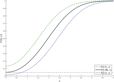
where F(c,|ν|) = 1 −Φ(c− |ν|) + Φ(−c− |ν|) with the standard normal cumulative
distribution function Φ(·).
3. Under Assumptions 3.2 and 3.5, following holds
lim sup
n→∞
P(InfTn(θ0)> cinf1−α)≤F(c inf
1−α,0), (4.6)
lim sup
n→∞
P(InfTn(θ0)> z1−α/2)≤α. (4.7)
Under Assumption 3.1 (same rates of K), Corollary 4.2.1 shows that the tests based
on InfTn(θ) asymptotically control size assuming all K ∈ Kn satisfy the undersmoothing
condition. As InfTn(θ0) ≤ |Tn(K, θ0)| and |Tn(K, θ0)| d
Kn, the test based on InfTn(θ) using normal critical value also controls the asymptotic
size, but conservative. Without undersmoothing assumption, Corollary 4.2.2 shows that
the asymptotic size is bounded above by the asymptotic size of a single t-statistic with the
smallest asymptotic bias infπ|ν(π)|. Note that F(c,|ν|) is a monotone decreasing in c and
increasing in |ν|. See also Hall and Horowitz (2013), Hansen (2014) for the similar function
and Figure 1 for the plots of F(·,·) as a function of|ν| with some different c.
Note that cinf1−α ≤ z1−α/2, so that F(z1−α/2,0) = α ≤ F(cinf1−α,0). Moreover, the upper
bounds of the asymptotic size can be small if the smallest bias infπ|ν(π)| is small. For
example, when cinf1−α = 1.5, F(cinf1−α,infπ|ν(π)|) = 0.13 for infπ|ν(π)| = 0. (4.5) also shows
that the test based on InfTn(θ0) with normal critical value controls size asymptotically if
the smallest bias is 0.
Under Assumption 3.5 (different rates of K), Corollary 4.2.3 shows that asymptotic size
of the tests based on InfTn(θ) is bounded above even when we allowing ‘large’ asymptotic
bias (|ν(m)|=∞) for several Ks in Kn.3
Remark 4.1 (LargestK). Although, there exist rate restrictions for ¯K by Assumption 3.2 to be used for the asymptotic normal approximation, formal guidance or data-dependent
results for the range of Kn = [K,K¯] are beyond the scope of this paper. Nevertheless,
the test based on InfTn(θ0) and its asymptotic critical value cinf1−α may have better power
compare with the test based on Tn(K, θ0) with the normal critical value for some large K.
Suppose that InfTn(θ0) = |Tn(K, θ0)| for some largeK (say ¯K) under the null, then the test
based on InfTn(θ0) may have better power as this test compares with the smaller critical
value than the normal critical value.
Also, note that the asymptotic size result in (4.7) relies on the inequality InfTn(θ0) ≤ |Tn( ¯K, θ0)| and the fact that Tn( ¯K, θ0)
d
−→ N(0,1) under Assumption 3.5. But, theory can provide the bound of the asymptotic size in (4.7) as F(z1−α/2,infm|ν(m)|) without any
undersmoothing conditions on K ∈ Kn. Asymptotic distribution result in Corollary 4.1.2
is still valid as long as infm|ν(m)| is bounded. If we know (a priori) that ¯K satisfies the
undersmoothing condition and others not, then there’s no point of searching over different
3If we further assume V1/2
K K
η, η > 0 for all K ∈ Kn then Σ = I
M and t-statistics are
asymptot-ically independent (see discussions below Theorem 3.2). Then, we can get asymptotic size of the test as
QM
m=1F(c inf
1−α,|ν(m)|). The asymptotic size is not affected byKm such that|ν(m)|=∞sinceF(c,∞) = 1
for any constantc >0. Further, suppose that the lastM1 number ofKs satisfy undersmoothing conditions and the others satisfy oversmoothing rates, i.e., |ν(m)| = ∞ for m = 1,· · ·, M −M1 and |ν(m)| = 0 for the others. Then, the asymptotic size is equal to αM1/M, ascinf
1−α = z1−α1/M/2 follows from Theorem 3.2
and Σ =IM. In this special case, the asymptotic size is a decreasing function of the fraction of number of
K; we may just use ¯K for the inference. This may work well if ¯K coincides with some
size-optimal sequence K∗(n) = arg minK|P(Tn(K, θ0) > z1−α/2)− α|. However K∗(n) is
unknown, so the choice of ¯K can be ad hoc in practice.
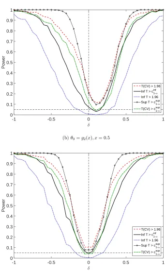
Remark 4.2 (Power of the test). Although InfTn(θ) leads to the tests that control the
asymptotic size or bound the size distortions, one reasonable concern is that possible low
power property of the test compare with the other statistics (e.g., the supremum of the
t-statistics). Investigating local asymptotic power comparisons of the level α test based
on several different statistics, or some optimal property of the tests in this nonparametric
regression context is important, but these are beyond the scope of this paper. I discuss the
length of CIs based on inverting an infimum test statistic in Section 5. I also report the
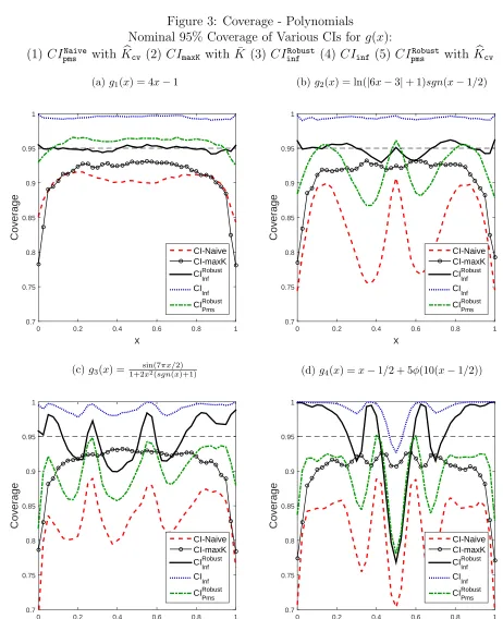
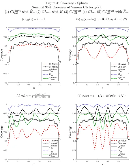
length of proposed CIs (Figures 5-6) and power of the tests (Figure 7) in Section 8 with various simulation setups.
The goal of this paper is to develop tests which can control size distortions even allowing
large asymptotic bias for several different series approximations. I want to emphasize that
bias issues can severely affect commonly used inference procedures (i.e., coverage of standard
CI) in series estimation. For example, high-order polynomials can be highly sensitive to the
choice of series terms. Using low-order polynomials or regression splines can help to reduce
bias issues, but does not solve bias problem completely. Moreover, a test based on the other
transformation of the t-statistics can be sensitive to the bias problems, thus may lead to
size distortions of the tests. For example, see Appendix C for the inference based on the supremum test statistic under Assumption 3.5.
4.3
Critical values
In this section, I discuss detail descriptions to approximate critical values defined in (4.2).
Here, I suggest using simple simulation methods to obtain critical values. To make implemen-tation procedures simple, I impose following set assumption and conditional
homoskedastic-ity.
Assumption 4.1. (Set of finite number of series terms)
Kn ={K ≡ K1,· · ·, Km,· · ·,K¯ ≡KM} where Km = πmK¯ for constant πm, 0< π =
π1 < π2 <· · ·< πM = 1, fixed M, and K¯ = ¯K(n)→ ∞ as n→ ∞.
Assumption 4.2. (Conditional homoskedasticity) E(ε2
i|xi =x) = σ2.
Assumption 4.1 is a finite dimensional version of Assumption 3.1 and is different with an
of generality, we assume K1 < K2 < · · ·< KM and they are all integers. In finite samples,
we only consider finite setKn, so the difference between Assumption 4.1 and 3.5 only matters
in large samples. Conditional homoskedasticity assumption is only for a simpler
implemen-tation. Based on the general covariance structure defined in Theorem 3.1 and 3.2, we can
construct a variance-covariance matrix using its sample analogs under the heteroskedastic
error.
By Theorem 3.1, following finite dimensional convergence of the t-statistics holds under
the Assumptions 3.2, 3.4, 4.1, and 4.2
(Tn(K1, θ0),· · ·, Tn(KM, θ0))0 d
−→Z = (Z1,· · ·, ZM)0, Z ∼N(0,Σ), (4.8)
where Σ is a variance-covariance matrix, Σjl = limn→∞VK1/2j /VK1/2l for any j and l, provided
that Σ exists and is a finite positive definite matrix. (4.8) also holds under same assumptions
as in Theorem 3.2. Note that the limiting distribution does not depend on θ0 and
variance-covariance matrix Σ can be consistently estimated by its sample counterparts. This requires
estimators of the varianceVKthat are consistent uniformly overK ∈ Kn. Define least square
residuals as εbKi =yi−PKi0 βbK, and let VbK as the simple pluig-in estimator for VK
b
VK =PK(x)0Qb−K1ΩbKQb−K1PK(x),
b QK =
1
n
n
X
i=1
PKiPKi0 , ΩbK =
1
n
n
X
i=1
PKiPKi0 εb
2
Ki.
(4.9)
Then, I define bcinf
1−α based on the asymptotic null distribution of InfTn(θ0) as follows,
b
cinf1−α≡(1−α) quantile of inf
m=1,···,M|Zm,Σb|,
whereZ
b
Σ = (Z1,Σb,· · ·, ZM,Σb) 0 ∼
N(0,Σ)b , Σbjj = 1,Σbjl=Vb
1/2
Kj /Vb
1/2
Kl .
(4.10)
One can compute bcinf
1−α by simulating B (typically B = 1000 or 5000) i.i.d. random vectors
Zb b
Σ ∼N(0,Σ) and by taking (1b −α) sample quantile of{InfT b
n = infm |Zm,b Σb
|:b = 1,· · ·, B}.4
I impose following assumption on the consistency of variance estimator VbK uniformly in
K ∈ Kn.
Assumption 4.3. sup
K∈Kn
|VbK
VK −1|=op(1) as n, K → ∞.
4Under heteroskedastic error terms, we can construct
b
Σj,l =
b
VKjl
b
V1/2
Kj Vb1/2
Kl
for any j < l, where VbKjl is an
sample analog estimator ofPKj(x)
0E(P
KjiP
0
Kliε
2
i)PKl(x) andVbKj,VbKlare estimator of the varianceVKj, VKl,
Assumption 4.3 is satisfied under same regularity conditions (Assumption 3.1 and 3.2)
with an additional assumption. For example, if we further assume sup
K∈Kn
||Pn
i=1P˜KiP˜
0
Kiε2i −
E[ ˜PKiP˜Ki0 ε2i]||=op(1) with an orthonormalized vector of basis functions ˜PK(x)≡Q
−1/2
K PK(x),
then Assumption 4.3 holds. See Lemma 5.1 of Belloni et al. (2015), and also Lemma 3.1
and 3.2 of Chen and Christensen (2015b) for different sufficient conditions under mild rate
restrictions and unconditional moment of the error terms.
Next, we consider a t-statistic Tn,Vb(K, θ) = q n
b
VK(
b
θK −θ0) replacing variance of the
series estimatorVK with VbK. Following Corollary provides the joint asymptotic distribution
of Tn,Vb(K, θ) for K ∈ Kn and the validity of Monte Carlo critical values bc
inf
1−α defined in
(4.10).
Corollary 4.3. Under Assumptions 3.2, 3.4, 4.1, 4.2 and 4.3,
(Tn,
b
V(K1, θ0),· · ·, Tn,Vb(KM, θ0)) 0 d
−→Z
where Z = (Z1,· · ·, ZM)0 ∼N(0,Σ) with a positive definite matrix Σ defined in (4.8). This
also holds under the Assumptions 3.2, 3.4, 3.5, 4.2, and 4.3. Furthermore, bcinf 1−α
p −→ cinf
1−α
holds where bcinf
1−α is defined in (4.10) and cinf1−α is the (1−α) quantile of inf
m=1,···,M|Zm|.
Remark 4.3(Weighted bootstrap). Alternatively, we can use the weighted bootstrap method to approximate asymptotic critical values. Implementation of the weighted bootstrap method
is as follows. First, generate i.i.d draws from exponential random variables {ωi}ni=1,
inde-pendent of the data. Then, for each draw, calculate LS estimator weighted by ω1,· · ·, ωn for
each K ∈ Kn and construct weighted bootstrap t-statistic as follows
ˆ
βKb = arg min
b
1
n
n
X
i=1
ωi(yi−PKi0 b) 2, gˆb
K(x) =PK(x)0βˆKb ,
Tnb(K) =
√
n(ˆgKb (x)−gˆK(x))
b
VK1/2 .
(4.11)
Then, construct InfTb
n = infK|Tnb(K)|. Repeat thisB times (1000 or 5000) and definebc
inf,W B 1−α
as conditional 1−α quantile of {InfTb
n : b = 1,· · ·, B} given the data. Similar to Belloni
et al. (2015), the idea behind the weighted bootstrap methods is as follows: if the limiting
distribution of weighted bootstrap process is equal to the original process conditional on
the data, then the weighted bootstrap process InfTnb also approximate the original limiting
distribution infπ∈[π,1]T(π). However, the validity of the weighted bootstrap is beyond the
5
Confidence interval
Now, I introduce confidence intervals for θ0 = g0(x) and provide their coverage properties.
We consider a confidence interval based on inverting a test statistic for H0 :θ =θ0 against
H1 : θ 6= θ0. Define CIinfRobust as the nominal level 1 −α CI for θ based on infimum test
statistics,
CIRobust
inf ≡ {θ : inf
K∈Kn
|Tn,Vb(K, θ)| ≤bcinf1−α}
={θ :|Tn,Vb(K, θ)|>bcinf1−α,∀K}C = [
K∈Kn
{θ :|Tn,Vb(K, θ)| ≤bcinf1−α}
= [inf
K(
b θK−bc
inf
1−αs(θbK)),sup
K
(θbK+ bc
inf
1−αs(θbK))]
(5.1)
where bcinf1−α is the Monte Carlo critical value defined in Section 4.3, s(θbK) ≡
q
b
VK/n is a
standard error of series estimator θbK usingK series terms, andAC denotes the complement
of a set A. Note thatCIRobust
inf can be easily obtained by using estimatesθbK, standard errors
s(θbK), and a critical value bc
inf
1−α. CIinfRobust is the lower and the upper-end point of confidence intervals for all K ∈ Kn using critical valuebc
inf 1−α.
Similarly, I define CIinf based on InfTn(θ) and the normal critical valuez1−α/2,
CIinf ≡ {θ: inf
K∈Kn
|Tn,
b
V(K, θ)| ≤z1−α/2}
= [inf
K (θbK−z1−α/2s(θbK)),supK (θbK +z1−α/2s(θbK))]
(5.2)
Note thatCIinfis the union of all confidence intervals forK ∈ Knusing conventional normal
critical value z1−α/2.
Next Corollary shows valid coverage property of the above CIs, and it follows from
Corollary 4.2 and 4.3.
Corollary 5.1. 1. Under Assumptions 3.2, 3.4, 4.1, 4.2, and 4.3,
lim inf
n→∞ P(θ0 ∈CI
Robust
inf ) = 1−α, lim infn→∞ P(θ0 ∈CIinf)≥1−α. (5.3)
2. Under Assumptions 3.2, 4.1, 4.2, 4.3, and supm|ν(m)|<∞,
lim inf
n→∞ P(θ0 ∈CI
Robust
inf )≥1−F(c
inf
1−α,infm |ν(m)|), (5.4)
lim inf
3. Under Assumptions 3.2, 3.5, 4.2, and 4.3,
lim inf
n→∞ P(θ0 ∈CI
Robust
inf )≥1−F(c
inf
1−α,0), (5.6)
lim inf
n→∞ P(θ0 ∈CIinf)≥1−α. (5.7)
Corollary 5.1.1 shows the validity of CIRobust
inf , i.e., asymptotic coverage is equal to 1−α.
The asymptotic coverage of CIinf is greater or equal than 1−α. Note that the Corollary 5.1.1 requires undersmoothing condition, i.e., no asymptotic bias for allKs in Kn.
Without undersmoothing assumption, Corollary 5.1.2 and 5.1.3 show that the coverage
probability of CIRobust
inf and CIinf are bounded below by the coverage of single K with the smallest asymptotic bias, similar to the asymptotic size results in Corollary 4.2. For example,
the lower bound in (5.6) is 0.87 whencinf
1−α = 1.5. Furthermore, (5.7) shows thatCIinf using standard normal critical value achieve nominal coverage probability 1−α. CIinfandCIinfRobust
bound coverage distortions even when we allow large asymptotic bias terms (|ν(m)| = ∞)
for severalKs in Kn. In this sense, CIinf and CIinfRobust are robust to the bias problems.
AlthoughCIinf gives formally valid coverage allowing asymptotic bias, coverage property of the CIinf in (5.3) and (5.7) holds with inequality; thus it can be conservative. As the
variance of series estimator increases with K, we expect CIinf can be comparable to the
standard CI using normal critical values with some largeK around ¯K. In contrast,CIRobust inf
has shorter length by using smaller critical value than the normal critical value.
Remark 5.1 (Length of the interval and the ranges ofK). Note that potential large length of theCIRobust
inf is also related to the possible low power property of the test. Also, note that
the last equality from the definition ofCIRobust
inf in (5.1) holds only when there is no dislocated
CI, i.e., the intersection is nonempty at least for some two CIs using bcinf1−α. Otherwise, using
the superset widens the length of CI. As the variance of series estimator increases with K, we expect that the union of all confidence intervals may only be determined by some large
Ks so that there is no dislocated CI. In general, dislocated confidence interval may show
some evidence of significant bias for some specific models, but there is no guarantee that the
union of the confidence interval is connected in practice.
Although this paper does not consider the data-dependent choice of Kn, a possible large
length of CI can be avoidable if K is reasonably large and this is exactly the condition
needed in Corollary 5.1 to have a correct coverage. Furthermore, the net effect of increasing
largest ¯K on the length ofCIRobust
inf is not clear as it may decrease critical valuesbc
inf
6
Post model selection inference
In this section, I provide methods to construct a valid CI that gives correct coverage after
selecting the number of series terms considering supremum of the t-statistics.
I first consider the ‘post model selection’ t-statistic
|Tn(K, θb )|, Kb ∈ Kn
whereKb is a possibly data-dependent rule chosen fromKn. Then, we define following ‘naive’
post-selection CI with Kb using the normal critical valuez1−α/2,
CINaive
pms ≡ {θ:|Tn(K, θb )| ≤z1−α/2}= [bθKb −z1−α/2s(θbKb),θbKb +z1−α/2s(bθKb)]. (6.1)
Conventional method of using normal critical values in (6.1) comes from the asymptotic
normality of the t-statistic under deterministic sequence, i.e., when Kn ={K}. However, it
is not clear whether the asymptotic normality of the t-statistic Tn(K, θb 0)
d
→ N(0,1) holds with some random sequence of Kb. Even if we assume the asymptotic bias is negligible, the
variability of Kb introduced by some selection rules can affect the variance of the asymptotic
distribution. Thus, it is not clear whether naive inference using standard normal critical
value is valid. If the post model selection t-statistic, Tn(K, θb 0) with some Kb, has
non-normal asymptotic distribution, then the naive confidence intervalCINaive
pms may have coverage
probability less than the nominal level 1−α.
Furthermore, Kb with some data-dependent rules may not satisfy the undersmoothing
rate conditions which ensure the asymptotic normality without bias terms. For example,
suppose a researcher uses Kb = Kbcv selected by cross-validation. It is well known that
the Kbcv is typically too “small” so that lead to a large bias by violating undersmoothing
assumption needed to ensure asymptotic normality and the valid inference. If Kb increases
not sufficiently fast as the undersmoothing condition does, then the asymptotic distribution
may have bias terms and resulting naive CI may have large coverage distortions.
Here, I construct a valid post-selection CI with Kb ∈ Kn by adjusting standard normal
critical value to the critical value from a ‘supremum’ test statistic,
SupTn(θ)≡ sup
K∈Kn
|Tn(K, θ)|. (6.2)
Note that |Tn(K, θb 0)| ≤ SupTn(θ0) for any choice of Kb ∈ Kn, and SupTn(θ0) d
−→ ξsup ≡
supπ∈[π,1]|T(π)| under the same assumptions as in Corollary 4.1. Therefore, inference based
will be valid, but conservative. Similar to cinf
1−α defined in (4.2), I define asymptotic critical
valuecsup1−α as 1−α quantile of ξsup. We can approximate this critical value by using Monte
Carlo simulation based method similarly as in Section 4.3. To be specific, I define
b
csup1−α ≡(1−α) quantile of sup
m=1,···,M
|Zm,
b
Σ|, (6.3)
whereZΣb = (Z1,Σb,· · ·, ZM,Σb)0 ∼N(0,Σ) andb Σ are defined in (4.10). We can verifyb bc
sup 1−α
p −→
csup1−α similar to Corollary 4.3.
Next, I define the following robust post-selection CI using the critical value bcsup1−α rather
than the normal critical value z1−α/2 compare to CIpmsNaive,
CIpmsRobust≡[θb
b
K −bc
sup 1−αs(θb
b
K),bθ
b
K+bc
sup 1−αs(bθ
b
K)], Kb ∈ Kn. (6.4)
Next Corollary shows that the robust post-selection CIRobust
pms guarantees the asymptotic
coverage as 1−α. Even though Corollary 6.1 does not implicitly use randomness of the
specific data-dependent selection rules of Kb, CIpmsRobust can be useful as it can be applied to
any selection rules among Kn.
Corollary 6.1. Under Assumptions 3.2, 3.4, 4.1, 4.2, and 4.3,
lim inf
n→∞ P(θ0 ∈CI
Robust
pms )≥1−α. (6.5)
(6.5) also holds under Assumptions 3.2, 3.4, 3.5, 4.2 and 4.3.
Corollary 6.1 imposes an undersmoothing (Assumption 3.4) and does not allow optimal
MSE rates (e.g.,Kbcv). ThusCIpmsRobustdoes not deal with the bias problem explicitly. However,
it accommodates bias by enlarging confidence interval using larger critical values bcsup1−α than
the normal critical value. Moreover, we also expectbcsup1−αis smaller than the usual
Bonferroni-type critical value. Bonferroni corrections use normal critical value z1− α
2M replacing α with α/M. However, Bonferroni critical value can be too large especially when|Kn|=M is large,
as it ignores dependence structure of the t-statistics.
7
Extension: partially linear model setup
In this section, I provide inference methods for the partially linear model (PLM) similar to
the nonparametric regression setup.
Suppose we observe random samples {yi, wi, xi}ni=1, where yi is scalar response variable,
variables. For simplicity, we shall assume wi is a scalar. I consider following partially linear
model
yi =θ0wi+g0(xi) +εi, E(εi|wi, xi) = 0. (7.1)
We are interested in inference on treatment/policy effectθ0 after approximating unknown
function g0(x) by series terms/regressorsp(xi) among a set of potential control variables. A
number of regressors can be large if there are many available control variables, i.e.,p(xi) =xi
or if there are large number of transformations of p(xi) are available such as polynomials
and interactions of xi. For notational simplicity, I use the similar notation as defined in
nonparametric regression setup. Suppose we useK regressorsPKi=PK(xi), wherePK(x) =
(p1(x),· · ·, pK(x))0 from the basis functions p(x). The approximating model can be written
as
yi =θ0wi+PKi0 βK+εKi, (7.2)
where the error term εKi = rKi +εi and approximation error rKi are defined similarly as
in Section 2. Then, series estimator θbK for θ0 using the first K approximating functions is
obtained by standard LS estimation of yi onwi and PKi, and has the usual “partialling out”
formula
b
θK = (W0MKW)
−1
W0MKY (7.3)
where W = (w1,· · ·, wn)0, MK = IK −PK(PK
0
PK)−1PK0, PK = [P
K1,· · ·, PKn]0, Y = (y1, · · ·, yn)0. Similar to the nonparametric regression model, we are interested in testing for
H0 :θ =θ0 againstH1 :θ 6=θ0.
The asymptotic normality and valid inference for the partially linear model have been
developed in the literature. Donald and Newey (1994) derived the asymptotic normality of
b
θK under standard rate conditions where K/n→0. See also Robinson (1988), Linton (1995)
and references therein for the related results of the kernel estimators. Belloni, Chernozukhov, and Hansen (2014) analyzed asymptotic normality and uniformly valid inference for the
post-double-selection estimator even when K is much larger than n under some form of
sparsity condition. A recent paper by Cattaneo, Jansson, and Newey (2015a) provided a
valid approximation theory forθbK even when K grows at the same rate of n.
Different approximation theory using faster rate of K (K/n → c > 0) than the
stan-dard rate conditions (K/n → 0) is particularly useful for our purpose to better reflect the
![Figure 2: Different functions of(10(x −) used in simulations (Section 8).gg·4(x) = x − 1/2 + 5φ23 g(xSolid lines (Black) are g1(x) = 4x − 1; Dashed lines (Green) areg2(x) = ln(|6x − 3| + 1)sgn(x − 1/2); Dotted lines (Blue) are(x) = sin(7πx/2)/[1 + 2x(sgn(x) + 1)]; and Dash-dot lines (Red) are 1/2)), where φ() is the standard normal pdf.](https://thumb-us.123doks.com/thumbv2/123dok_us/9371639.439802/58.612.114.500.84.373/figure-dierent-functions-simulations-section-dashed-dotted-standard.webp)