The development of solid state NMR methodology to study the dynamics of proteins and ice

warwick.ac.uk/lib-publications

A Thesis Submitted for the Degree of PhD at the University of Warwick

Permanent WRAP URL:

http://wrap.warwick.ac.uk/126885

Copyright and reuse:

This thesis is made available online and is protected by original copyright.

Please scroll down to view the document itself.

Please refer to the repository record for this item for information to help you to cite it.

Our policy information is available from the repository home page.

M A

E

G NS

I MOLEMT A T

U N IV

E R SIT_{AS WAR WI}C EN S

I S

The Development of Solid-State NMR Methodology

to Study the Dynamics of Proteins and Ice

by

Rebecca A. Stevens

Thesis

Submitted to the University of Warwick

for the degree of

Doctor of Philosophy

Department of Chemistry

Contents

Acknowledgments vi

Declarations vii

Abstract viii

List of Tables ix

List of Figures x

List of Abbreviations xiv

List of Symbols xvi

Chapter 1 Introduction 1

Chapter 2 Theory 6

2.1 Solid-State NMR Fundamentals . . . 6

2.1.1 Nuclear Spins . . . 6

2.1.2 NMR Interactions . . . 8

2.1.3 Magic Angle Spinning . . . 11

2.2 Pulsed Fourier Transform NMR . . . 12

2.2.1 The Basic SSNMR Experiment . . . 12

2.2.2 The Rotating Frame . . . 14

2.2.3 Cross Polarisation . . . 14

2.2.4 Proton Detection . . . 17

2.2.5 Heteronuclear Decoupling . . . 17

2.2.6 Solvent Suppression . . . 17

2.2.7 Isotopic Labelling . . . 18

2.2.8 Basics of 2D NMR Experiments . . . 21

2.3 Relaxation Theory . . . 23

2.3.1 The Origins of Relaxation . . . 23

2.3.2 The Correlation Time, Correlation Function and Spectral Density Function . . . 24

2.3.4 Spin-Lattice Relaxation (R1) . . . 30

2.3.5 Spin-Spin Relaxation (R2) . . . 32

2.3.6 Spin-Lattice Relaxation in the Rotating Frame (R1ρ) . . . 32

2.3.7 The Model Free Approach . . . 33

2.3.8 Relaxation Experiments . . . 34

2.3.9 Relaxation Dispersion Measurements . . . 39

2.3.10 Temperature and Relaxation . . . 39

2.3.11 The Nuclear Overhauser Effect . . . 42

2.3.12 Chemical Exchange . . . 42

2.3.13 Spin Diffusion . . . 43

2.3.14 Chemical Exchange Saturation Transfer . . . 45

2.3.15 Cross-Correlated Relaxation . . . 47

2.4 Solid-State NMR Applied to Biological Samples . . . 47

2.4.1 Protein GB1 . . . 48

Chapter 3 Development of Tools to Aid the Packing of Proteins into Solid-State NMR Rotors 50 3.1 Abstract . . . 50

3.2 Introduction . . . 50

3.3 Literature Review . . . 53

3.4 Design and Development of the Packing Tools . . . 56

3.4.1 Initial Packing Tools for 1.3 mm Rotors . . . 56

3.4.2 First Development: Creating a Fixed Rotor to Swinging Bucket Adaptor . . . 61

3.4.3 Initial Tests for 1.3 mm Packing Tools . . . 61

3.4.4 Second Development: Creating Rotor Sleeves for 0.7 and 0.8 mm SSNMR Rotors . . . 62

3.4.5 Third Development: Adapting the Rotor Sleeves and Funnel for 0.7 and 0.8 mm SSNMR Rotors to Avoid Leaks . . . 64

3.4.6 The Final Design of the Ultracentrifuge Tools . . . 64

3.5 Using the Tools to Pack Samples . . . 68

3.5.1 Packing a Microcrystalline Protein Sample for NMR . . . 68

3.5.2 Sedimentation and Packing of a Protein Sample . . . 68

3.6 Experimental Considerations for Sedimentation . . . 71

3.6.1 The Concentration and Molecular Weight Requirements for Suc-cessful Protein Sedimentation . . . 71

3.6.2 Calculating the Time Required to Sediment a Protein Sample Us-ing the MLS-50 and MLA-150 PackUs-ing Tools . . . 74

3.7 Conclusions and Outlook . . . 74

3.8 Experimental Details . . . 77

3.8.1 Information on the Ultracentrifuge . . . 77

3.8.3 Testing of the Tools . . . 77

3.8.4 Protein Samples . . . 79

3.8.5 NMR Experiment(s) . . . 79

Chapter 4 1H-Detected NMR Measurements of Aliphatic 13C R1 in Fully-Protonated Proteins in the Solid State 81 4.1 Abstract . . . 81

4.2 Introduction . . . 82

4.3 Literature Review . . . 82

4.3.1 Spin Diffusion . . . 82

4.4 Results . . . 86

4.4.1 Spin Diffusion Control Spectra at 60 and 100 kHz MAS . . . 88

4.4.2 Spin Diffusion Saturation Transfer at 100 kHz MAS . . . 91

4.4.3 Experimental 13CR1 Measurements at Variable MAS . . . 92

4.4.4 Cross-Correlated Relaxation . . . 100

4.5 Conclusions and Outlook . . . 100

4.6 Experimental Details . . . 103

4.6.1 Protein Samples . . . 103

4.6.2 SSNMR Experimental Details . . . 103

4.6.3 Determination of Relaxation Rates . . . 108

Chapter 5 Variable-Temperature, Solid-State NMR Measurements to Investigate the Site-Specific Relaxation and Energy Landscape of GB1109 5.1 Abstract . . . 109

5.2 Introduction . . . 110

5.3 Results . . . 112

5.3.1 Variable TemperatureR1 andR1ρ Measurements . . . 112

5.3.2 Use of the Extended Model Free Approach to Determine Order Parameters, Correlation Times and Activation Energies . . . 117

5.4 Conclusions and Outlook . . . 124

5.5 Experimental Details . . . 129

5.5.1 Protein Samples . . . 129

5.5.2 Assignment . . . 129

5.5.3 SSNMR Experimental Details . . . 129

5.5.4 Determination of Relaxation Rates . . . 131

5.5.5 EMF-Arrhenius Analysis of the 13C’ and15N R1 and R1ρ . . . 131

5.5.6 Monte Carlo Error Analysis . . . 132

Chapter 6 Investigating the Effects of “Antifreeze” Molecules on Ice Growth Using Solid-State NMR 133 6.1 Abstract . . . 133

6.3 Terminology . . . 134

6.4 Literature Review . . . 137

6.4.1 Binding Sites of AF(G)Ps . . . 139

6.4.2 Is AF(G)P-Ice Binding Reversible? . . . 142

6.4.3 Proposed Mechanisms for the Antifreeze Effect(s) of AF(G)Ps on Ice . . . 143

6.4.4 Research into Antifreeze Proteins and Ice by Solid-State NMR . . 146

6.4.5 AFGP8, North Atlantic Pout AFP and Barfin Plaice AFP . . . 147

6.4.6 Synthetic Antifreezes . . . 148

6.4.7 Negative Controls . . . 152

6.4.8 Applications of AFPs, AFGPs and Synthetic Antifreezes . . . 153

6.5 Results . . . 154

6.5.1 Variable Temperature1_HR 1 of Ice in the Presence of Antifreezes . 155 6.5.2 Variable Temperature1HR2 of Ice in the Presence of Antifreezes . 158 6.5.3 Variable Temperature1H Relaxation Dispersion of Ice in the Pres-ence of Antifreezes . . . 163

6.5.4 2D 1H-1H EXSY Spectra . . . 166

6.5.5 Discussion . . . 168

6.6 Conclusions and Outlook . . . 170

6.7 Experimental Details . . . 172

6.7.1 Antifreeze Samples . . . 172

6.7.2 Temperature Calibration . . . 172

6.7.3 NMR Experimental Details . . . 173

Chapter 7 Summary and Outlook 177 Appendices 181 Appendix A Theory 182 A.1 Assignments of Protein GB1 . . . 182

A.2 Calculating the Effect of Spin Diffusion on PDSD . . . 184

Appendix B Development of Tools to Aid the Packing of Proteins into Solid-State NMR Rotors 185 B.1 Detailed Protocol for the Ultracentrifuge Packing Tools . . . 185

B.1.1 Sedimenting Samples: . . . 185

B.1.2 Packing a Crystalline Sample into a Rotor: . . . 189

B.2 Sedimentation Calculations . . . 191

Appendix C 1H-Detected NMR Measurements of Aliphatic 13C R1 in

Appendix D Variable-Temperature, Solid-State NMR Measurements to Investigate the Site-Specific Relaxation and Energy Landscape of GB1199

D.1 13C’ and15NR1andR1ρPlotted Against the Inverse Absolute Temperature199

D.2 Calculation of the Correlation Times, Order Parameters and Activation Energies from 13C’ and 15N R1 and R1ρ . . . 205

Appendix E Investigating the Effects of “Antifreeze” Compounds on Ice

Growth Using Solid-State NMR 209

Acknowledgments

First and foremost, I would like to thank my supervisor, Dr. J´ozef Lewandowski, not

only for his invaluable guidance and unremitting enthusiasm, but also for providing me

with many opportunities to travel, both across the UK and internationally, in order to

present my work and attend workshops. I am also extremely grateful for the countless

hours he has spent teaching me over the last 4 years.

I would also like to thank all of those who have helped me with SSNMR

measure-ments and analysis, or produced protein samples, in particular Dr. Jonathan Lamley,

Dr. Carl ¨Oster, Dr. Trent Franks, Dr. Angelo Gallo, Dr. Simone Kosol and Sarah

Mann. Additionally, I would like to express my gratitude towards Dr. Andy Howes and

Dr. Gregory Rees for their technical assistance. Huge thanks go to Alice Fayter for all

her work in the antifreeze project, whom it was truly a pleasure to collaborate with,

and I would like to thank Christopher Stubbs and Dr. Muhammad Hasan for providing

the PVA samples and antifreeze proteins. Financial support from the EPSRC is also

gratefully acknowledged.

On a personal note, I am extremely grateful to past and present members of the

Warwick Solid-State NMR group for the many friendships over the years that have made

this PhD the experience it was. I’ve thoroughly enjoyed the climbing, board games and

excessive amounts of cake! I will miss you all. Additionally, I will always be grateful

for the fantastic teachers I have had throughout school, sixth form and university for

sparking my interest in the sciences and truly inspiring me, I wouldn’t be where I am

today without them.

Special thanks go to my family for supporting me in everything I do, despite not

always understanding what I do or why I do it. Finally, I am indebted to Seb for his

superior grasp of the English language, attention to detail and his best attempts to keep

Declarations

The work in this thesis is original, and was conducted by the author, unless otherwise

stated, under the supervision of Dr J´ozef R. Lewandowski (Department of Chemistry).

The work has not been submitted for a degree or diploma or other qualification at

any other University. Funding was provided by an EPSRC studentship. All sources of

information have been acknowledged by means of reference throughout the text.

All collaborative results are indicated in the text, a brief summary is given here:

The initial designs for the 1.3 mm rotor packing tools presented in Chapter 3

were developed by Dr W. Trent Franks and Georgina Charlton, supervised by Dr J´ozef

Lewandowski. Later developments stemmed from discussions with Dr W. Trent Franks

and Koorosh Fatemian. All versions of the tools were manufactured by Lee Butcher and

Marcus Grant in the Department of Chemistry’s mechanical workshop (University of

Warwick).

The SDST measurements presented in Chapter 4 were performed by Dr.

An-gelo Gallo and the 60 kHz MAS PDSD spectra were recorded with guidance from Dr.

Jonathan Lamley (both supervised by Dr. J´ozef R. Lewandowski).

All of the work presented in Chapter 6 is in collaboration with Alice Fayter,

supervised by Professor Matthew I. Gibson (Department of Chemistry, University of

Warwick). The PVA samples were synthesised by Christopher Stubbs and the AFPs by

Abstract

Solid-state nuclear magnetic resonance (SSNMR) is an excellent tool for determin-ing the molecular motions within a dynamic system. SSNMR relaxation measurements can access a vast range of timescales (ps - ms) and are able to simultaneously determine the frequency and amplitude of the motion that a particular nucleus is undergoing.

Recent developments in SSNMR instrumentation now allow for>100 kHz magic

angle spinning (MAS) using 0.7 and 0.8 mm rotors. State-of-the-art MAS is especially beneficial for those wishing to investigate proteins in the solid state: only sub-milligram amounts of sample are required and the fast spinning yields incredible spectral resolution. This also enables proton detection and the associated improvements in sensitivity (for protonated samples). Unfortunately, these small rotors are extremely challenging to pack with the semi-solid protein samples. Furthermore, the proteins can become dehydrated in the slow packing process, making them unsuitable for NMR. To address this point, in Chapter 3, we present the design and application of an ultracentrifuge tool for the packing of proteins into 0.7 - 1.3 mm diameter SSNMR rotors. The tool helps to reduce the waste of expensive isotopically labelled proteins and decreases the packing time from several hours to minutes.

The work in Chapter 4 takes advantage of the mentioned fast MAS developments and demonstrates the accurate measurement of site-specific, spin-lattice relaxation rates (R1) on 13Cα nuclei in a fully protonated, uniformly 13C-labelled protein at 100 kHz

MAS. Our approach overcomes the averaging effect of proton-driven spin diffusion that obscures site-specific information for the relaxation rates measured at slower spinning frequencies.

One area where measurements of relaxation in the solid state can yield significant insights is the understanding of the complex energy landscape describing conformational changes of proteins, which are often closely linked to their functions. In Chapter 5 we present some of the first extensive site-specific variable temperature measurements of 13C’ and 15N R1 and spin-lattice relaxation rates in the rotating frame (R1ρ) in a

crystalline protein as a way to explore its conformational energy landscape. We observe

R1ρ more than doubling over a narrow range of temperatures and minimal variation

in R1 over the same range. We model the relaxation data using an extended model

free approach and Arrhenius relationship to extract activation energies for the motions dominating the dynamics, however find that further measurements are required for an accurate determination of the activation energies.

In Chapter 6 we show that relaxation measurements in the solid state are not

only useful for characterising protein motions. In this chapter, we employ variable

List of Tables

2.1 Common nuclei for NMR. . . 7

2.2 GB1 sequence. . . 49

3.1 Details on packing tools in the literature. . . 55

3.2 Ultracentrifuge conditions for using the tools. . . 68

3.3 Example minimum concentrations required for sedimentaion of various proteins. . . 73

3.4 Example sedimentation coefficients and times. . . 75

3.5 Maximum ultracentrifuge speeds and forces. . . 77

3.6 Testing conditions for the MLA-150 packing tool. . . 79

3.7 Testing conditions for the MLS-50 packing tool. . . 80

4.1 Conditions for VMAS measurements on (U-1H,13C,15N)GB1. . . 106

4.2 Conditions for VMAS measurements on (2-13C(glucose),U-1H,15N)GB1. . 107

5.1 Bond lengths . . . 120

5.2 Sample temperatures . . . 131

6.1 Colligative antifreezes. . . 134

6.2 AFPs and the ice planes they bind to. . . 139

6.3 PVA MWs and PDIs . . . 172

A.1 The 1H,13C and15N assignments for crystalline GB1. . . 183

B.1 Parameters required for calculating whether sedimentation would be ef-fective. . . 192

List of Figures

1.1 Timescales of dynamic proccesses and NMR techniques. . . 2

1.2 Magic Angle Spinning . . . 3

2.1 CSA . . . 10

2.2 Magic Angle Spinning . . . 12

2.3 ‘One-pulse’ NMR experiment. . . 13

2.4 Fourier transform of an FID. . . 13

2.5 The laboratory and rotating frames. . . 14

2.6 Example of a cross polarisation pulse sequence. . . 16

2.7 The [1,3-13C]glycerol and [2-13C]glycerol labelling schemes. . . 19

2.8 The [2-13C]glucose labelling scheme. . . 20

2.9 A 1D and a 2D spectrum of protein GB1. . . 22

2.10 Example of a 2D pulse sequence. . . 22

2.11 Relaxation processes. . . 23

2.12 Correlation function and spectral density function. . . 25

2.13 Transition probabilities in a two-spin system. . . 27

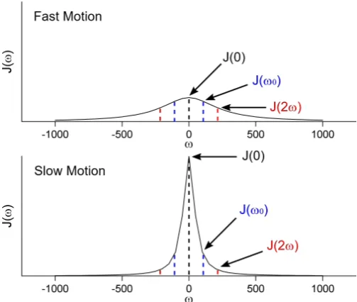
2.14 Example spectral densities at ω = 0, ω0 and 2ω0. . . 29

2.15 R1 . . . 31

2.16 R2 . . . 32

2.17 R1ρ . . . 33

2.18 Example R1 pulse sequence using the Torchia method. . . 36

2.19 1H saturation recovery R1 pulse sequence. . . 37

2.21 R2 pulse sequence . . . 38

2.22 Effect of the the spin-echoes in a 1_HR 2 CPMG pulse sequence. . . 38

2.23 R1ρ . . . 40

2.24 Examples of R1ρ and RD plots. . . 40

2.25 Variation in R1 and R2 with correlation time. . . 42

2.26 SD simulations. . . 46

2.27 CEST . . . 46

2.28 Protein GB1 . . . 48

3.1 Different techniques for the preparation of protein samples for SSNMR. . 52

3.3 Previous packing method for 0.7 and 0.8 mm rotors. . . 52

3.4 Old method for packing proteins into rotors. . . 53

3.5 Ultracentrifuge tools in the literature. . . 55

3.6 The fixed rotor and swinging bucket ultracentrifuge rotors. . . 57

3.7 Packing with different ultracentrifuge rotors. . . 57

3.8 Initial packing tools. . . 59

3.9 Diagram of initial tools. . . 60

3.11 Future improvement for the adaptor. . . 61

3.10 Dimensions and photos of the adaptor. . . 62

3.12 Illustrations of different rotor sleeves - initial design. . . 63

3.13 Reasons for the tool leaking. . . 65

3.14 Ideas for better adapting the tool for 0.7 and 0.8 mm rotors. . . 65

3.15 Illustrations of different rotor sleeves - final design. . . 66

3.16 Photograph and illustration of packing tools. . . 67

3.17 Illustration of steps for using the tool. . . 69

3.18 Comparison of spectra of protein packed using the packing tools and a spatula. . . 70

3.19 A diagram of the ultracentrifuge tool parameters. . . 72

3.20 Conditions for successful sedimentation using the packing tools. . . 73

3.21 Time required for complete sedimentation. . . 75

3.22 Technical drawing of the swinging bucket MLS-50 tool, fixed angle MLA-150 tool and the adaptor. . . 78

4.1 Dipolar interactions in a protein. . . 84

4.2 2H-labelling . . . 84

4.3 Partial13C-labelling. . . 85

4.4 2D13C-1H at 100 kHz MAS. . . 87

4.5 PDSD spectra at 60 kHz . . . 89

4.6 RFSD spectra at 60 kHz . . . 90

4.7 Control PDSD spectra at 100 kHz MAS. . . 91

4.8 Example SDST profiles. . . 93

4.9 13Cα _{SDST profiles for residues 1 - 32. . . . 94}

4.10 13Cα _{SDST profiles for residues 33 - 56. . . . . 95}

4.11 The13_C-13_{C chemical shift difference between the neighbouring} 13_Cα _and sidechain nuclei. . . 96

4.12 Example 13Ca VMAS plots. . . 97

4.13 VMAS 13_Cα _R 1 measured in fully-protonated, uniformly-labelled crys-talline GB1. . . 97

4.14 13CR1 measured in fully-protonated, uniformly-labelled crystalline GB1 . 98 4.15 VMAS 13Cα _R 1 for uniformly and partially 13C-labelled GB1. . . 99

4.17 PDSD and RFSD pulse sequences. . . 104

4.18 A 1H-13C-1H PDSD control pulse sequence. . . 104

4.19 13C SDST pulse sequence. . . 105

4.20 13CR1 pulse sequence. . . 107

5.1 Example energy landscape and timescale of motions within a protein. . . 111

5.2 13C’ and15NR1 andR1ρ at 28.0°C. . . 113

5.3 VT 13_{C’ and} 15_{N R} 1. . . 115

5.4 VT 13C’ and 15N R1ρ. . . 116

5.5 Correlation times, order parameters and activation energies from the EMF analysis. . . 122

5.6 Reproducing the13C’ and 15N R1 and R1ρ rates at 34.85°C. . . 125

5.7 Reproducing relaxation rates that were not involved in the initial model. . 126

5.8 1_H-15_{N assignments. . . 130}

5.9 Pulse sequences used for 13C’ and 15N R1 and R1ρ. . . 130

6.1 Ih structure and the conditions for other phases of ice. . . 136

6.2 Planes of ice. . . 136

6.3 Ostwald ripening. . . 136

6.4 Dynamic Ice Shaping . . . 137

6.5 Quasi-liquid layer. . . 138

6.6 AFGP structure. . . 138

6.7 Examples of AFPs from a range of organisms. . . 140

6.8 Regularly ordered threonine groups on AFPs. . . 140

6.9 DIS . . . 142

6.10 Examples of AFP I binding planes. . . 143

6.12 Adsorption-inhibition mechanism. . . 144

6.13 Adsorption-inhibition models for ice growth in the presence of AF(G)P. . 145

6.14 The anchored clathrate water mechanism. . . 146

6.15 AFPIII interaction with its hydration shell and ice. . . 147

6.16 Structure of AFGP8 and North Atlantic Pout AFP III. . . 148

6.17 Structure of PVA. . . 149

6.18 PVA binds to primary and secondary prism planes of ice. . . 149

6.19 Effect of PVA concentration and DP on the IRI activity of PVA. . . 151

6.20 Structure of safranin chloride, phenosafranin chloride and safranin nitrate. 151 6.21 Structure of PEG and lysozyme. . . 153

6.22 VT R1 of ice in the presence of antifreezes and controls. . . 156

6.23 VT R2 of ice in the presence of antifreezes and controls. . . 160

6.24 The contributions toR2. . . 161

6.25 VT R2 of ice in the presence of PVA at different concentrations. . . 162

6.26 VT RD of ice in the presence of proteins. . . 164

6.28 VT RD of ice in the presence of dyes. . . 165

6.29 2D 1H-1H EXSY measurements . . . 167

6.30 2D 1H-1H EXSY measurements on liquid samples. . . 169

6.31 Summary of SSNMR measurements on ice in the presence of various an-tifreezes. . . 169

6.32 Temperature calibration using methanol. . . 173

6.33 The pulse sequence for measurement of 1H R1. . . 174

6.34 The pulse sequence for measurement of 1H R2. . . 175

6.35 The pulse sequence for measurement of 1H R1ρ. . . 175

6.36 The pulse sequence for measurement of 2D 1_{H EXSY spectra. . . 176}

C.1 All VMAS spectra. . . 194

C.2 VMAS 13Cα _R 1 . . . 195

C.3 VMAS 13_Cα _R 1 continued. . . 196

C.4 Sidechain VMAS 13CR1 . . . 197

D.1 VT 13C’ R1 . . . 200

D.2 VT 13C’ R1ρ. . . 201

D.3 VT 15N R1 . . . 202

D.4 VT 15N R1ρ . . . 203

D.5 VT 13CR1 sidechains . . . 203

D.6 VT 13CR1ρ sidechains . . . 204

D.7 VT 15N R1 sidechains . . . 204

D.8 VT 15N R1ρ sidechains . . . 205

E.1 1D 1H spectra of 1 mg/ml DP150 PVA solution freezing. . . 210

E.2 1D 1_{H spectra of AFGP . . . 210}

E.3 1D 1H spectra of Lysozyme . . . 211

E.4 1D 1H spectra of PVA . . . 211

E.5 1D 1_{H spectra of PEG . . . 212}

E.6 1D 1H spectra of Safranin . . . 212

List of Abbreviations

AFGP(s) Antifreeze Glycoprotein(s)

AFP(s) Antifreeze Protein(s)

CD Circular Dichroism

CEST Chemical Exchange Saturation Transfer

CFRP Carbon Fibre Reinforced Polymer

CP Cross Polarisation

CPMG Carr-Purcell-Meiboom-Gill

Cryo-EM Cryogenic Electron Microscopy

CSA Chemical Shift Anisotropy

DIS Dynamic Ice Shaping

DSC Differential Scanning Calorimetry

DSS 4,4-Dimethyl-4-Silapentane-1-Sulphonic Acid

DP Degree of Polymerisation

EMF Extended Model Free

EPR Electron Paramagnetic Resonance

EXSY Exchange Spectroscopy

FA Fixed Angle (Ultracentrifuge Rotor)

GB1 Immunoglobulin Binding Domain B1 of Streptococcal Protein G

Ih Hexagonal Ice

IBS Ice-Binding Site

IR Infrared spectroscopy

IRI Ice Recrystallisation Inhibition

ISP Ice-Structuring Protein

MAS Magic Angle Spinning

MD Molecular Dynamics

MF Model Free

MLA-150 Fixed Angle Ultracentrifuge Rotor (Speed ≤150,000 rpm)

MLGS Mean Largest Grain Size

MLS-50 Swinging Bucket Ultracentrifuge Rotor (Speed ≤50,000 rpm)

MRI Magnetic Resonance Imaging

MW Molecular Weight

NMR Nuclear Magnetic Resonance

NOE Nuclear Overhauser Effect

PBS Phosphate-Buffered Saline

PCTFE Polychlorotrifluoroethylene

PDI Polydispersity Index

PDSD Proton Driven Spin Diffusion

PEEK Polyether Ether Ketone

PEG Polyethylene Glycol

Phenosafranin Phenosafranin Chloride

POM Polyoxymethylene

PVA Polyvinyl Alcohol

PVP Poly(N-Vinyl Pyrrolidone)

QLL Quasi-Liquid Layer

RAFT Reversible Addition-Fragmentation Chain Transfer

RD Relaxation Dispersion

RF Radio Frequency

RFSD RF-Driven Spin Diffusion

Safranin Safranin Chloride

SAXS Small-Angle X-Ray Scattering

SB Swinging Bucket (Ultracentrifuge Rotor)

SD Spin Diffusion

SDST Spin Diffusion Saturation Transfer

SMF Simple Model Free

SNR Signal-to-Noise Ratio

SSNMR Solid-State Nuclear Magnetic Resonance

TF Freezing Point

TH Thermal Hysteresis

TM Melting Point

TOCSY Total Correlation Spectroscopy

TTMSS Tris(trimethylsilyl)silane

VMAS Variable Magic Angle Spinning

VT Variable Temperature

VTU Variable Temperature Unit

List of Symbols

D Dipolar Interaction

I Spin Angular Momentum

R Gas Constant

R1 Spin-Lattice Relaxation Rate

R1ρ Spin-Lattice Relaxation Rate in the Rotating Frame

R2 Spin-Spin Relaxation Rate

S Svedburg Unit (10-13 _s)

S2 Order Parameter

T1 Spin-Lattice Relaxation Time

t1 Indirect Evolution Time

T1ρ Spin-Lattice Relaxation Time in the Rotating Frame

T2 Spin-Spin Relaxation Time

t2 Direct Evolution Time

h Planck Constant

¯

h Reduced Planck Constant

γ Gyromagnetic Ratio

µ Magnetic Moment

µ0 Vacuum Permeability Constant

σ Proton Driven Spin Diffusion Exchange Rate

Chapter 1

Introduction

Over the last few decades significant developments in solid-state nuclear magnetic

res-onance (SSNMR) have moulded it into a extremely powerful technique for the

deter-mination of dynamics in wide range of proteins, including challenging systems, such as amyloid fibrils1–3 and large non-crystalline protein-protein complexes.4–6 Proteins are

incredibly complex biomolecules that perform an impressive range of functions in living

cells and are critical for life. One of the huge challenges facing biologists is the determi-nation and understanding of protein functions. Vast amounts of research has focused on

the relationship between protein function and structure. However these biomolecules are

not rigid, they are highly flexible and undergo continual fluctuations in their conforma-tions, thus a stationary structure can only represent a weighted average of the possible

confirmations. It is a combination of the proteins structure and dynamics that

ulti-mately determine its function. Furthermore, dynamics are crucial for various biological processes, such as ligand binding, enzymatic catalysis and protein folding.7–9

Research into the dynamics of proteins can be challenging due to the vast range of timescales upon which these may occur (see Figure 1.1).10 _{Over the years, nuclear}

magnetic resonance (NMR) has developed into an ideal technique for investigating

pro-tein dynamics at atomic-resolution on almost all functionally-relevant timescales. NMR has the ability to probe all (NMR-active) nuclei within a protein simultaneously, but

can also selectively focus on specific regions. With suitable experimental set-up and

resolution it is possible to individually monitor each nucleus within the protein, whereas most analytical techniques can either focus on only a few specific sites (e.g. fluorescence

microscopy) or observe an average response from the entire protein (e.g. neutron

diffrac-tion). Historically, most proteins were investigated using solution-state NMR. Recent advances in SSNMR methodology and equipment, combined with the fact that many

proteins are insoluble or too large to monitor in the solution state, have made the use

of SSNMR extremely valuable. It has been questioned whether proteins prepared for SSNMR accurately represent the native environment, but there is increasing evidence

The very first solid-state and solution-state NMR spectra were reported in 1946 by Purcellet al.18 and Blocket al.,19 respectively. Ever since, solution-state measurements

have dominated the field due to an inherent advantage of rapidly tumbling molecules,

allowing various anisotropic interactions, which would otherwise cause extremely broad peaks, to be averaged out. Whereas solid samples have restricted motion and producing

broad, often difficult to interpret, peaks in the spectra. Independently, Andrew et al.20

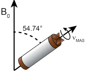
and Lowe21 realised that this problem might be mitigated by macroscopic rotation of the solid in a way which mimics the tumbling of a solution. As described in Section

2.1.3 and Figure 1.2, fast rotation of the solid sample at a 54.7° angle with respect to the strong magnetic (B0) field can sufficiently narrow the peaks. Faster spinning at this

“magic angle” improves the averaging out of the anisotropic interactions and so narrows

the linewidths. However, there are technical limits to achievable spinning speeds. Most modern rotors are made of zirconia and have decreased in diameter over the years as

magic angle spinning (MAS) technology has advanced. The first rotor designed by

Andrew et al. had an outer diameter of 8 mm and would spin at a maximum of 0.83

kHz. Now it is common to use 4 mm to 1.3 mm (external diameter) rotors that have

maximum spinning speeds of 10 kHz to 70 kHz.22 Furthermore, state-of-the-art MAS

uses 0.7 mm rotors that are capable of spinning at 110 kHz.

The rapid developments in MAS are especially beneficial for those wishing to

investigate proteins in the solid state. Proteins are often costly and challenging to

produce and so are typically available only in milligram amounts. Therefore these 0.7 mm rotors, which are filled by sub-milligram amounts of sample, are ideal, providing

that sufficient sensitivity can be achieved. More importantly, the fast spinning aids

obtaining excellent spectral resolution. For example it becomes possible to conduct proton-detected experiments on protein samples, which results in achieving significant

gains in sensitivity that often compensates for the small sample size.23–25

The spectra obtained at extremely fast MAS are impressive, but the smaller SSNMR rotors have made the packing of protein samples increasingly challenging. The

sub-milligram amounts of protein are too sticky to be packed into a rotor using a spatula

Figure 1.2: An SSNMR rotor spinning at the “magic angle” (54.74° from the B0 field)

or other standard tools, but also too viscous to be packed using a pipette. Most labs use home-made contraptions involving various pipette tips and a benchtop centrifuge to force

their protein into the rotor, often a long-winded process. The longer the process takes,

the higher the chance of the valuable protein sample becoming dehydrated, rendering it unsuitable for NMR. In response to this, in Chapter 3, I present the design and

application of an ultracentrifuge tool for the packing of such samples into 0.7 - 1.3 mm

diameter SSNMR rotors. The tool helps to reduce the waste of expensive isotopically labelled proteins and decreases the packing time from several hours to minutes.

There are further benefits to the development of such fast MAS. The work in Chapter 4 demonstrates the measurement of certain dynamics within a protein that

would not be possible without 100 kHz MAS. The spin-lattice relaxation rate is

partic-ularly important for learning about fast, ps - ns motions, but the main challenge when measuring this type of relaxation is the suppression of an effect called “spin diffusion”.

Spin diffusion causes the magnetisation of neighbouring sites to exchange via dipolar

couplings, which averages out the measured relaxation rates so that they are no longer site-specific. Fast spinning is an important technique for decreasing the effects of spin

diffusion (via averaging the dipolar couplings). It is often combined with specific isotopic

labelling schemes and deuteration to make sure that spin diffusion is negligible during relaxation measurements. However, for some nuclei in certain systems, spin diffusion can

be particularly challenging to remove. This is the case for aliphatic nuclei in proteins

due to their strong1H-13C and13C-13C dipolar couplings. It is possible to measure the spin-lattice relaxation rates of aliphatic sites using extensive deuteration, partial 13C

labelling and 60 kHz MAS, however it can be very expensive and often challenging to

isotopically label proteins in this way. Thus, with the recent development of 100 kHz MAS, Chapter 4 investigates whether the spin-lattice relaxation rates of aliphatic 13C

nuclei, in particular 13Cα_{, can simply be measured with 100 kHz MAS in a fully}

proto-nated and uniformly 13C labelled protein. Alongside the relaxation rate measurements themselves, spin diffusion control spectra and spin diffusion saturation transfer (SDST)

measurements were conducted to analyse the extent of spin diffusion at the aliphatic

sites under these conditions. The13Cα _{nuclei throughout the protein backbone were}

es-pecially interesting because they are not part of the rigid peptide plane and thus undergo

dynamics distinct from the13C’ and15N backbone sites.

Relaxation measurements are one of the most powerful SSNMR tools since they allow simultaneous measurement of the timescale, amplitude and occasionally

direc-tionality of each motion.16, 26, 27 The “model free” approach, developed by Lipari and Szabo in 1982, is a very popular method for accurate estimation of the order

param-eters (i.e. effective amplitudes) and correlation times (i.e. effective timescales) of the

motions from relaxation rate data.28, 29 This approach is used extensively in Chapter 5. Figure 1.1 summarises the dynamics commonly found within protein samples and the

timescale upon which they occur. Each type of relaxation measurement is sensitive to

motions on the ps - ns timescale, such as methyl group rotations. Whereas spin-spin relaxation rates are sensitive to slower dynamics (ns - ms), such as local folding.

To-gether this hierarchy of dynamics forms the overall energy landscape of the protein and

its function(s).7, 9, 30 SSNMR relaxation measurements across a range of temperatures are well-suited for characterising the hierarchy of protein dynamics, since the

combi-nation of the Arrhenius equation and the model free approach allow the quantitative

determination of activation energies. Chapter 5 explores the use of 13C’ and 15N vari-able temperature relaxation measurements to further understand the energy landscape

throughout a protein backbone.

Relaxation rates are not only extremely valuable for determining the motions

within a protein, they can be applied to many other dynamic systems. The research

in Chapter 6 investigates the use of variable temperature relaxation measurements and 2D exchange spectra to determine the ice dynamics within frozen non-colligative

an-tifreeze solutions. Non-colligative anan-tifreezes are those that depress the freezing point

of water significantly more than predicted by concentration alone. Since the first ob-servation of antifreeze glycoproteins in polar fish, many more antifreeze glycoproteins

and antifreeze proteins have been discovered across a vast range of organisms. These

naturally-occurring antifreezes are extremely effective at very low concentrations and are vital for the survival of many species in cold habitats. Considering the huge

quan-tities of research on these complicated proteins, relatively little is known about their

mechanism for such effective antifreeze activity. The applications of these impressive biomolecules are vast and spread across the biomedical, agricultural and engineering

industries. However, these proteins are challenging and costly to produce in significant

quantities, so synthetic mimics of antifreeze (glyco)proteins are extremely sought after. Only a handful of synthetic antifreezes have been discovered and as such there is

lim-ited knowledge of their mechanisms too. In this work, the dynamics of frozen aqueous

solutions of antifreeze (glyco)proteins and two synthetic mimics, polyvinyl alcohol and safranin chloride, are explored using SSNMR. In the literature there is little use of

SS-NMR to explore such systems. Moreover, the majority of measurements focus on the

antifreezes themselves, whereas this research monitors changes in the motions of the ice protons in the presence of the antifreezes. This chapter aims to develop the knowledge of

ice-antifreeze dynamics and aid the determination of a mechanism, complementing the

research from other techniques, such as splat assays, nanolitre osmometry, fluorescence microscopy and molecular dynamics simulations.

The research presented in this thesis starts with an important practical consideration

for SSNMR of proteins, the development of a packing tool (Chapter 3). It is followed by two chapters focusing on advancing SSNMR methodology for the determination of

protein dynamics (Chapters 4 and 5) and finally, in Chapter 6, similar techniques are applied to investigate the dynamics of ice in the presence of various non-colligative

Chapter 2

Theory

In order to understand the results presented in this thesis, a basic knowledge of SSNMR

and relaxation theory is required. In this light, this chapter starts with a walk-through

of the fundamentals of SSNMR theory and followed by a section on the specifics of relaxation and relaxation measurements.

Large amounts of the theory presented here come fromUnderstanding NMR

Spec-troscopy (J. Keeler),31Spin Dynamics (M. H. Levitt),32NMR(P. J. Hore),33NMR: The Toolkit(P. J. Hore, J. Jones and S. Wimperis),34Solid-State NMR: Basic Principles and

Practice(D. C. Apperley, R. K. Harris and P. Hodgkinson),35Introduction to Solid-State

NMR Spectroscopy (M. Duer)36and SSNMR Studies of Biopolymers (A. E. McDermott and T. Polenova).37

2.1

Solid-State NMR Fundamentals

One of the most important differences between NMR in the solid state and in the solu-tion state is the lack of rapid overall mosolu-tion in solids. In a solusolu-tion the molecules are

tumbling very quickly and undergoing random motions, therefore any NMR parameters

that are orientation dependent (anisotropic) will be averaged out to their orientation independent (isotropic) values, but in the solid state this is not the case. Thus a

pri-mary challenge when measuring dynamics using SSNMR is separating the incoherent

contributions (due to random motions) from the coherent contributions (due to incom-plete averaging of anisotropic interactions). Many experiments have been designed and

developed to address this and these will be discussed in Section 2.3, but first the basic concepts and key interactions of SSNMR are described.

2.1.1 Nuclear Spins

All atomic nuclei possess three important physical properties: mass, electric charge and spin. The latter is an intrinsic angular momentum, critical for NMR. The overall

magnitude of the spin of a nucleus is determined by the spin quantum number (I), which

is a positive integer or half integer (I = 0,1₂,1,3₂,2...). The spin quantum number of common nuclei are presented in Table 2.1. Note that isotopes with I = 0, such as 12C,

Table 2.1: Common nuclei and their spin quantum numbers, gyromagnetic ratios, natural

abundances and Larmor frequencies at 14.1 T (600 MHz1H Larmor frequency).

Nucleus Spin (I) Natural

Abundance (%)

Gyromagnetic Ratio (MHz T-1)

Larmor Frequency at 14.1 T (MHz)

1_{H 1/2 99.98 42.577 600.0}

2_{H 1 0.02 6.536 92.1}

12_{C 0 98.9 N/A N/A}

13_{C 1/2 1.1 10.708 150.9}

14_{N 1 99.6 3.077 43.3}

15_{N 1/2 0.4 -4.316 60.8}

All nuclei with a non-zero spin quantum number are inherently magnetic, they

possess a magnetic moment (µ):

µ=γIz (2.1)

Where γ is the gyromagnetic ratio, a constant of proportionality between the angular

momentum (Iz) and the magnetic moment. γ has a different value for each type of

nucleus. Iz is the angular momentum of these spin states, which is quantised as:

Iz=m¯h (2.2)

Wherem=I, I−1, I−2, ...,−I+ 1,−I.

All NMR-active nuclei have 2I + 1 spin states. The nuclei studied in this work

(1H, 13C and 15N) are all spin I = ₂1, therefore each has two states: mI = +1₂¯h and

mI = −1₂¯h. In these cases the lower energy state will be aligned with the external

magnetic field (B0), known as the αspin state (mI = +1₂¯h) and the higher energy state

will be aligned against the magnetic field, known as theβspin state (mI =−1₂¯h), ifγis

positive.

Each of the spin states has an energy associated with it (Equation 2.3):

EZ =−γm1¯hB0 (2.3)

The energy difference between these spin state relates to a transition between

these states (Equation 2.4), this is known as theZeeman effect.

|∆EZ|=|γ¯hB0| (2.4)

These transitions are critical for NMR. They can be related to a resonance

fre-quency for NMR, known as the Larmor frequency (ω0), through equations 2.5 and 2.6:

∆EZ = ¯hω0 (2.5)

WhereB0 is the applied magnetic field strength. Note that in the NMR community the

spectrometers are often referred to by their 1H Larmor frequency rather than their B0

field strength. For example, 600 MHz rather than 14.1 T.

The energy difference between spin states can be used to calculate the proportion of nuclear spins in theαand βstates (i.e. aligned with or against the external magnetic

field) at thermal equilibrium:

pβ

pα

=e∆kTEZ (2.7)

Where pβ

pα is the ratio of spins in the βand αstates,k is the Boltzmann constant andT is temperature.

When describing NMR experiments, it is often much more convenient to consider

the behaviour of the net magnetisation (also called the “bulk magnetisation”) rather

than considering individual spins. Unfortunately the net magnetisation is extremely small meaning that NMR is a very insensitive analytical technique. For example, in the

case of13C nuclei at aB0 field of 9.4 T, for every 1,000,000 spins in theβstate there will

only be 1,000,017 in the α state. Due to its inherently poor sensitivity a lot of research has been dedicated to developing techniques to improve the signal-to-noise ratio (SNR)

of NMR experiments, these will be discussed in detail further on.

In this work the hydrogen, carbon and nitrogen nuclei are used as probes to investigate proteins and ice since these are the most abundant elements in these systems. These

elements have multiple isotopes and so the choices behind studying 1H (rather than

2_H), 13_{C (rather than} 12_{C) and} 15_{N (rather than}14_{N) are outlined below. The natural}

abundances, gyromagnetic ratios and calculated Larmor frequencies at a field strength

of 14.1 T are presented in Table 2.1 for these isotopes.

1_{H nuclei have a very high natural abundance and gyromagnetic ratio. The}

com-bination of these properties results in a relatively high signal-to-noise ratio. Alternatively

2_{H could be used, however the natural abundance of} 2_{H is very low (0.02%), therefore}

2_{H labelling would be necessary which can be expensive and challenging. Furthermore,}

2_{H has a gyromagnetic ratio 6.5 times smaller than that of}1_{H, resulting in a much lower}

signal-to-noise ratio. It is also a quadrupolar (spin >1/2) which results in significantly broader signals. 12C is by far the most abundant isotope of carbon, however it has a

spin quantum number of zero and therefore is NMR-inactive. This leaves 13C (1.1 %

abundance), which often calls for the sample to be isotopically labelled to achieve a good signal in reasonable experimental time. 15N is the most suitable isotope of nitrogen for

these experiments due to14N being quadrupolar. However, 15N has a very low natural

abundance (0.36%) and so isotopic labelling is usually required.

2.1.2 NMR Interactions

It is important to understand some of the key NMR interactions that affect the Lar-mor frequency of a nucleus. These are briefly described here. Each interaction will have

inter-action is on the scale of hundreds of MHz, dipolar coupling and chemical shift anisotropy are both on the scale of tens of kHz and J-couplings are typically 1-100 Hz.

ω0 ≈Zeeman+Dipolar+CSA+ChemicalShielding+J-Coupling (2.8)

The precise Larmor frequency of nucleus in a magnetic field does not just depend

upon the type of nucleus (i.e. gyromagnetic ratio), but also the environment surrounding

it. Local magnetic fields induced by currents of electrons in the molecular orbitals will slightly shield nearby nuclei from the B0 field, this well-known effect is calledchemical

shift or chemical shielding. It is one of the most important effects in solution-state

NMR for the determination of chemical structure. The chemical shift, like the Larmor frequency, is proportional to the external magnetic field. So it is practical to describe

the chemical shift in terms of its ratio to the Larmor frequency, thus providing an

instrument-independent description:

δ(ppm) = ω0−ω0,REF

ω0,REF

×106 (2.9)

Where δis the chemical shift (in parts per million), ω0 is the Larmor frequency of the

nucleus of interest andω0,REF is the Larmor frequency of a reference compound exposed

to the same external magnetic field.

In most cases, electrons are not spherically distributed around a nucleus, therefore shielding from the electrons will be anisotropic. This means that the orientation of

the nucleus with respect to the B0 field will affect the chemical shift, this is known

as chemical shift anisotropy (CSA). In the solution state, where the molecules are rapidly tumbling through all orientations, this anisotropy is averaged out and just the

isotropic chemical shift is observed. But in the solid state CSA is an important factor to

consider because the molecules will be in a variety of orientations with respect to the B0

field, and each will produce a slightly different chemical shift. The resulting peak will

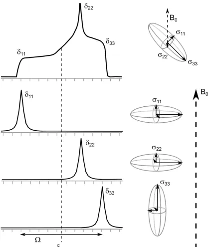
be a superposition of all possible orientations and therefore have a broad characteristic shape. The CSA tensor of this lineshape can be described by three components: δ11,

δ22 and δ33, which are defined as δ11 ≥ δ22 ≥ δ33 (i.e. the δ11 component corresponds

to the direction of highest shielding and theδ33component corresponds to the direction

of lowest shielding).38 _{A nucleus is described as being “axially symmetric” if two of the}

components are equal. The isotropic chemical shift is the mean of these three components

(Equation 2.10).

δiso=

δ11+δ22+δ33

3 (2.10)

Figure 2.1 illustrates the effect CSA can have on the chemical shift of a peak in the solid state.

Figure 2.1: The effect of CSA on a static powder sample. Theδ11,δ22andδ33components

are indicated, showing examples of how their orientation with respect to B0 can cause

patterns, which are very useful in the solution state for structure determination. In the solid state the effects of J-coupling are rarely resolved, because its interaction usually

has the smallest magnitude by far.

Dipolar coupling is a through-space interaction between a pair of dipole mo-ments. The secular approximation, valid in strong external magnetic fields, of the dipolar

coupling between two spins (D), j andk, is defined by Equation 2.11:

D=−µ0

4π γjγk¯h

r3

1 2(3 cos

2_θ

jk−1) (2.11)

Where µ0 is the magnetic moment, γj and γk are the gyromagnetic ratios of the spins,

r is the distance between the spins and θjk is the angle between the dipolar vector and

the B0 field.

Like CSA, this interaction is also anisotropic: each orientation will give a different splitting, which causes the overall NMR signal to become broad. It is important to note

that the dipolar interaction is strongly distance dependent, therefore a spin will have

the strongest dipolar interactions with those closest in space to it. It is also dependent on the gyromagnetic ratios of the involved nuclei, thus the strongest dipolar interactions

will involve 1H nuclei.

2.1.3 Magic Angle Spinning

It is routine to apply magic angle spinning (MAS) in SSNMR experiments to assist in

the removal of the line-broadening effects of CSA and dipolar couplings, which have a common dependence on orientation (at least to the first order approximation):

1 2(3 cos

2_{θ−1) (2.12)}

Whereθis the angle between the B0 field and the CSA principle axes or dipolar tensor.

Andrew20 and Lowe21 independently discovered that rotation of a solid sample at 54.74° to the B0 field reduces Equation 2.12 to zero on average (see Figure 2.2),

mimicking the tumbling of a solution sample:

1 2(3 cos

2_{54.74°−1) = 0 (2.13)}

This angle has been termed the “magic angle”. To effectively average CSA or dipolar interactions, the frequency of the magic angle spinning (MAS) has to be

signif-icantly larger than the size of the interaction. The extent of precisely how much faster

the spinning frequency needs to be is dependent on the nature of the interaction. For example, homonuclear dipolar couplings are typically more difficult to average out than

heteronuclear dipolar couplings (due to a difference in an element of the dipolar coupling

Hamiltonian when the chemical shifts of the coupled spins are similar i.e. in a

homonu-clear interaction).36 MAS of up to 60 kHz is typical in protein SSNMR experiments,

however more recent advances in NMR equipment now allow for MAS up to 150 kHz.

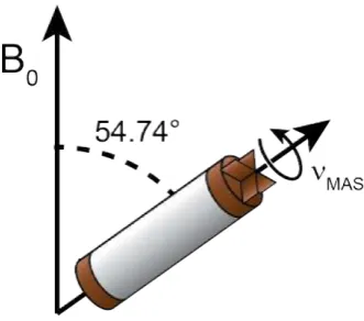
Figure 2.2: An SSNMR rotor spinning at the “magic angle” (54.74° from the B0 field)

at a frequency ofνM AS.

broadening, for example broadening caused by a distribution of isotropic chemical shifts due to structural inhomogeneity.39

2.2

Pulsed Fourier Transform NMR

2.2.1 The Basic SSNMR Experiment

The initial set up of an SSNMR experiment involves placing the sample (packed inside a rotor) into a strong external magnetic field (usually 10 - 20 Tesla). Around the rotor

there is a coil of wire for both the application of radiofrequency (RF) pulses to the

sample and the detection of signal. The strong B0 field causes the nuclear spins to align

either with or against the field, producing a very small net magnetic field (aligned with

the B0). It is this net magnetisation that is manipulated and detected in the NMR

experiments.

The simplest “one-pulse” NMR experiment is illustrated in Figure 2.3 as a bulk

magnetisation vector and as a pulse sequence. In this experiment the bulk magnetisation

vector starts on the z-axis aligned with the B0 field. Only magnetisation in the plane

perpendicular to B0 is detectable, therefore, to produce an NMR signal, an RF pulse

along they-axis is applied to rotate the bulk magnetisation by 90°into thexy-plane (i.e.

spins transition from the α to the β energy levels). The magnetisation vector will now precess around thez-axis in thexy-plane and induce a current in the coil that surrounds

the sample. The detected current will be a superposition of oscillations at the Larmor

frequencies of the observed spins over time (each nucleus in a unique environment will produce a slightly different frequency). This signal is called a free induction decay

(FID) and will decay over time due to relaxation, which is the process by which the system returns to equilibrium. The FID, a time-domain signal, is complicated to analyse

directly and so it is Fourier transformed to produce a frequency-domain spectrum,

Figure 2.3: The “one-pulse” NMR experiment represented as a) bulk magnetisation vectors and b) the pulse sequence (where the x-axis is time). The black rectangle rep-resents a 90°ypulse that rotates the magnetisation (grey arrow) into the xy-plane ready

for acquisition of the signal (damped sine wave).

Figure 2.4: A vector model of a) magnetisation on thez-axis and then b) precessing and returning to equilibrium after a 90° pulse. c) Detection during this period produces the FID (time-domain data), which is then Fourier transformed to d) an NMR spectrum (frequency-domain data).

S(ω) =

i=N X

i=1

S(t)e−iωti _(2.14)

Where S(ω) is the signal at frequency ω, N is the number of digital points recorded,

S(t) is the signal at timet,ti is the time of theith data point.

In the case of a 90° pulse, the signal at time t (i.e. the voltage induced in the

coil) can be described as:

S(t) =S0eiΩte−R2t (2.15)

Where R2 is the rate of decay of magnetisation in the xy-plane and Ω is the angle

between the bulk magnetisation and the axis.

The Fourier transform of Equation 2.15 is:

S(ω) = S0R2

(ω−Ω)2_+R2 2

+i −S0(ω−Ω) (ω−Ω)2_+R2

2

(2.16)

The left-hand term in Equation 2.16 is the real part, which is an absorption mode

Lorentzian lineshape, and the right-hand term is the imaginary part, which is an

dispersion mode Lorentzian lineshape. Usually the real part of the spectrum is pre-sented, however often the spectrum will neither be an absorption nor dispersion mode

Lorentzian lineshape due to an arbitrary initial phase of the signal. In this case the spec-trum can be corrected using either frequency-independent (also known aszero-order) or

seeUnderstanding NMR Spectroscopy31 orSpin Dynamics.32

Most NMR experiments are more complex than the one described in Figure 2.3,

normally with multiple pulses, transfer of the magnetisation between different types of

nuclei (e.g. cross polarisation) and evolution periods (for 2D or 3D spectra). The net magnetisation is manipulated by RF pulses of various lengths and powers. These two

variables can be controlled to produce pulses that cause the net magnetisation to move

by precise angles and at exact speeds. The relationship between pulse angle (θ), power of the RF pulse (B1), pulse length (τp) and gyromagnetic ratio (γ) is shown in Equation

2.17. Normally when setting up experiments, the length and power for a 90° pulse (for a particular nucleus) are determined experimentally and then any other pulses can be

calculated from this pulse.

θ=γB1τp (2.17)

2.2.2 The Rotating Frame

So far all diagrams of bulk magnetisation have been shown in the laboratory frame

with the coordinatesx,y andz but, since the magnetisation precesses around thez-axis,

this frame of reference is not ideal. Instead a new coordinate system will be used from

now on, which moves around the z-axis at the Larmor frequency. This means that any

spins precessing at exactly the Larmor frequency will appear still and any spins at a

slight variation of this frequency will only move very slowly. This new frame of reference

is known as therotating frame (Figure 2.5).

2.2.3 Cross Polarisation

The signal from an NMR experiment is intrinsically low and so often the same experiment

is repeated many times to increase the signal-to-noise ratio. Cross polarisation (CP)

is an important technique used to provide information on multiple types of nuclei (i.e. different isotopes) in a single experiment, it is also used to increase the SNR and decrease

experimental time. CP involves the transfer of magnetisation from the nuclei of one

Figure 2.5: An example of the laboratory and rotating frames in the case of

magneti-sation in the xy-plane relaxing back to thermal equilibrium. The path of the bulk

element to another, most commonly from the nuclei of an abundant isotope (e.g. 1H) to a more dilute isotope of interest (such as13C or15N). In the case of 100% magnetisation

transfer there will be a signal enhancement of γ

1_H

γX compared to direct excitation of the X nuclei. In this research 1H-13C and 1H-15N CPs are frequently used, these give theoretical signal enhancements of approximately 4 and 10, respectively. Note that the

enhancement actually achieved in the experiment does depend on quality of the set up

(i.e. the pulse powers and lengths chosen in the pulse sequence), type of CP used and the sample type. Normally the theoretical efficiency of CP is limited to approximately

60 % of γ

1_H

γX , but can be up to 100 % if particular adiabatic CP pulse sequences are used.40, 41

Using CP instead of direct excitation can potentially reduce experimental time.

After running the pulse sequence the magnetisation needs to fully relax back to

equi-librium before repeating the experiment. The time that this takes is sample dependent and known as the spin-lattice relaxation time(T1). At the end of a pulse sequence

there is always a wait time known as the recycle delay that allows plenty of time for

this relaxation. Often 1H T1s are much shorter than 13C or 15N T1s. In the case of

a 1H-X CP, the recycle delay is limited by the 1H T1 (not the T1 of the X nuclei), so

typically this experiment can be repeated faster than a direct excitation experiment. A final, very important, advantage of CPs is that it allows the transfer of

mag-netisation between different types of nuclei within an experiment. Therefore information

on these different nuclei and their relationships to each other can be gathered in a sin-gle experiment. This is a vital tool in many SSNMR experiments, for example protein

structure assignment sequences and dynamics measurements.

CPs are critical for the research presented in this thesis and many of the pulse se-quences used involve two or three. For example, in the case of measuring relaxation in

a protein sample a pulse sequence involving 1H, 15N and 13C could be used. The

mag-netisation starts on the abundant 1H nuclei and is transferred to the 15N nuclei using a CP and then, after an indirect acquisition period on the 15_{N, the magnetisation is}

transferred to the 13C nuclei for detection, producing a 2D15N-13C spectrum.

Before further explanation of how CP works, the term “spin-lock” must be

defined. A spin-lock pulse is simply a strong pulse applied along the same axis as the

magnetisation vector (e.g. if the magnetisation is along the x-axis then the pulse will

be applied along the x-axis). This strong pulse ensures that the magnetisation remains along the axis since the RF field strength will be greater than any of the typical offsets

that would normally cause deviation from this axis, for example coherent contributions.

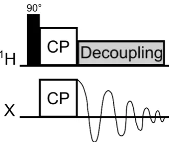
An example of a basic1H-X CP pulse sequence is shown in Figure 2.6. It starts with a

1_{H 90°pulse which brings the}1_{H spins from thez-axis into thexy-plane. Simultaneously,}

spin-lock pulses are applied on both the 1H nuclei and the X nuclei for a length of time

known as thecontact time(usually a few ms). Under the correct conditions, described below, the magnetisation will transfer from the 1H nuclei to the X nuclei during the

Figure 2.6: Example of a 1H-X cross polarisation pulse sequence. The x-axis is always time and each type of nucleus has its own row. The black narrow rectangle represents a 90° pulse, the two boxes labelled “CP” are the cross polarisation pulses, the damped sine wave represents the decay (and detection) of the X magnetisation and the grey box is the decoupling pulse.

acquisition time. (Further information on decoupling can be found in Section 2.2.5). During the contact time, both the 1H and X spins are spin-locked (into the xy

-plane). Naturally these nuclei will have different Zeeman splittings (energy difference

between the spin states). The1H and X spin-lock B1 fields can be applied in a way so

that they do have the same Zeeman splitting (quantised in B_x/y rather than B0), this

is known as the Hartmann-Hahn matching condition. Fulfilling the

Hartmann-Hahn condition (Equation 2.18) will cause both the 1H and X nuclei to have the same energy gap between their spin states, so that the 1H-X dipolar coupling allows a

re-distribution of energy between them. The fact that the net spin polarisation must be

preserved combined with the initial large1H magnetisation ultimately leads to a transfer of magnetisation from the1H to X nuclei.

γ1HB1₁H =γXB₁X (2.18)

Cross polarisation was originally developed for static SSNMR (i.e. without MAS).

Although the Hartmann-Hahn matching condition still holds for relatively slow MAS, if fast MAS is employed the spinning speed needs to be taken into account using Equation

2.19.

ν₁1H =ν₁X±nνM AS (2.19)

Where ν₁1H and ν₁X are the 1H and X nutation frequencies respectively, νM AS is the

MAS frequency and nis 1 or 2.

This highlights the importance of optimising the CP conditions at the target

MAS frequency to maximise the signal of the X nuclei. Under fast MAS the matching

conditions are much narrower, and inhomogeneity in the B1 fields can result in the

matching condition varying throughout the sample. Using ramped or adiabatic CP is

varied by sweeping the RF pulse through the matching condition, therefore achieving the matching condition for all parts of the sample at some point within the sweep. In

practice, using a ramped or adiabatic CP at high MAS frequencies tends to provide a

more intense signal and be more robust than a constant CP.40–42 It is for these reasons that adiabatic CPs are used throughout this work.

2.2.4 Proton Detection

It was mentioned that often a 1H-X experiment will be used to produce an X spectrum

instead of a direct X experiment because the extra magnetisation transferred from the

1_{H nuclei will significantly improve the signal. The overall sensitivity of the experiment}

also depends on which nucleus the magnetisation is detected. It generally improves if

it is detected on nuclei with a higher gyromagnetic ratio. In particular, experiments in

which the magnetisation is transferred from X to1H for detection provide large gains in sensitivity.43–46 Proton detectionis used throughout this work to improve sensitivity.

2.2.5 Heteronuclear Decoupling

If, during an NMR experiment, a dilute spin (for example 13_{C or} 15_{N) is observed}

while being surrounded by abundant spins (such as1H), heteronuclear dipolar coupling

will cause substantial broadening of the spectrum, even under fast MAS. It is common practice to incorporate specific RF pulses in the experiment in order to reduce this effect,

this is known asheteronuclear decoupling.

A technique commonly applied in this research, high-power heteronuclear decou-pling, involves applying continuous high-power RF irradiation on the 1H nuclei during

the FID acquisition of 13C, for example. The high-power pulse causes the 1H spins to

rapidly undergo repeated transitions between theαandβspin states at a rate determined by the RF pulse amplitude. If these spin state transitions are faster than the dipolar

coupling, the 13C spectrum will only be affected by the time-averaged dipolar coupling

which will be zero in this case due to the rapid spin-state oscillations of the 1H spins. At fast (> 50 kHz) spinning frequencies, where MAS is quite effective in removal of

heteronuclear couplings, low power decoupling sequences become viable and sometimes

even superior to high power approaches.47, 48

The specific types of decoupling used in these experiments (e.g. WALTZ-1649

and WALTZ-6450) are described in detail in the relevant experimental sections.

2.2.6 Solvent Suppression

Proton detection provides fantastic improvements in the sensitivity of SSNMR

experi-ments on proteins, however it comes coupled with intense1H signals from the solvent that overwhelm the spectra. In this work,Multiple Intense Solvent Suppression Intended for

Sensitive Spectroscopic Investigation of Protonated Proteins, Instantly (MISSISSIPPI)51

2.2.7 Isotopic Labelling

13_{C and} 15_{N Labelling}

As shown in Table 2.1, the natural abundance of many interesting isotopes is low, which

makes their NMR applications challenging. In this PhD project we investigated proteins and ice through measurements on the1H,13C and15N nuclei. 12C and 14N are far more

naturally abundant, however 12C is NMR-inactive and14N is quadrupolar, which poses

serious challenges in terms of resolution, sensitivity and general spin manipulation. The inherently low signal of NMR has already been discussed, but by probing extremely low

natural abundance isotopes (1.1 % and 0.4 %, respectively) this signal problem becomes

orders of magnitude worse.

One partial solution to this problem is to isotopically label the samples so that

they contain a much higher proportion of these13C and15N nuclei. Isotopic labelling is

achieved by expressing the proteins in minimal media with isotopically-labelled 13C or

15_{N sources, such as [U-}13_{C]-glycerol or [15%}15_{N]-ammonium chloride, as the sole carbon}

or nitrogen sources.52, 54–57 The specific isotopically-labelled 13C or 15N source chosen

defines the labelling in the resulting protein. It is common to use uniformly labelled sources to produce a [U-13C,15N] protein, but in some cases, such as those discussed

in Chapter 4, partial labelling is desirable to effectively turn “on” and “off” specific

interactions. For example, [1,3-13C]-glycerol or [2-13C]-glucose can be used to introduce

13_{C nuclei into specific sites within the protein. The presence of these isotopes at each}

particular site within each amino acid is well defined by a specific labelling scheme for each isotope source. The labelling schemes used in this work are presented in Figures

2.7 and 2.8.

Deuteration

Proton detection is a good method of improving sensitivity, since1H nuclei have a high

natural abundance and gyromagnetic ratio. Protons are also very abundant within

proteins, but this becomes a problem in the solid state: the dense network of 1H-1H dipolar couplings creates substantial line broadening, which offsets the advantages of

improved sensitivity. Often moderate MAS is combined with significant dilution of the

1_{H network with deuterium to reduce these linewidths. This is typically achieved by}

expressing the protein in deuterated media. Followed by exchanging of labile sites, such

as amide2Hs, by preparation in fully or partially protonated solvents.

The overall sensitivity obtained in deuterated samples is a balance between the level of dilution, resolution and sensitivity. As a rule of thumb, higher levels of dilution

are required for applications at slow spinning frequencies and larger fractions of protons

are tolerated at faster spinning frequencies.

Improvements in MAS technology have reduced the level of1H dilution required

for well-resolved, proton-detected spectra. Now as frequencies of 110 kHz MAS are

sample.

2.2.8 Basics of 2D NMR Experiments

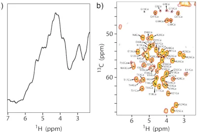
In biological samples, the 1H, 13C and 15N chemical shifts throughout the biomolecule all appear within a relatively small range, this leads to crowded spectra. For this reason

it is extremely rare to assign the structure of a biological sample using just a 1D

spec-trum, normally 2D and 3D spectra are needed. To illustrate this, examples of 1D and 2D spectra of the same protein sample are presented in Figure 2.9, the advantages of

multidimensional spectra are evident.

2D spectra can either be homonuclear or heteronuclear. An example of a basic homonuclear 2D pulse sequence is presented in Figure 2.10. After the initial 90° pulse,

there is a variable indirect evolution time (t1) in which the magnetisation evolves,

under the chemical shift of the first nucleus. Next there is a “mixing time” that allows magnetisation to exchange between nearby sites. Finally the NMR signal is detected as

a function of the time variablet2. Thisdirect evolution timeinvolves chemical shift

evolution on the second nucleus. The experiment is repeated many times incrementing t1 and then recording the FID as a function of t2. The dataset is Fourier transformed

twice (with respect to t1 and t2) to produce a 2D spectrum that is a function of both

frequency variables.58 A similar concept can be applied to produce 3D or nD spectra. In the case of multidimensional heteronuclear pulse sequences, the same concepts can

Figure 2.9: Examples of a) a 1D and b) a 2D spectrum of protein GB1. The sample is

uniformly 1H, 13C and 15N labelled. The spectra were recorded at 100 kHz MAS and

700 MHz1H Larmor frequency.