clouds of atoms in microtraps
Shimon Machluf,1 Julian B. Naber,1 Maarten L. Soudijn,1 Janne Ruostekoski,2 and Robert J. C. Spreeuw1
1Van der Waals-Zeeman Institute, Institute of Physics, University of Amsterdam,
Science Park 904, 1098XH Amsterdam, The Netherlands
2
Department of Physics, Lancaster University, Lancaster, LA1 4YB, United Kingdom
In this Supplemental material we provide a more de-tailed description of the numerical simulation methods that are used to demonstrate the density-dependent sup-pression of optical pumping. We also explain the image analysis we perform, and how we convert the optical den-sity image to number of atoms.
SIMULATION DETAILS
In the experiment the atoms are confined in an array of microtraps and occupy the (5S1/2) |F, mFi = |2,2i
electronic ground state. An incident laser excites the atoms to the (5P3/2)|F0, mF0i=|2,1istate from which the atoms decay to either the F = 2 manifold, with mF = 0,1,2 (of which mF = 0 is untrapped), or to
untrapped states in theF = 1 manifold, withmF = 0,1.
Reabsorption of light can take the atom to additional levels in the F = 1,2 and F0 = 2 manifolds. The opti-cal pumping rate is measured by detecting the remaining trapped atoms in theF = 2 states.
Standard coupled-dipole model simulations [1] are for-mulated for a single electronic ground level and for the limit of low light intensity where the atoms respond to light as linear harmonic oscillators. The system we are studying involves more than one electronic ground level that participate in optical transitions and the optical pumping necessitates simulation approaches that go be-yond the low light intensity limit, incorporating also the excited state dynamics. In order to do this we apply a recently proposed formalism [2] of coupled-dipole model equations that specifically account for the internal level dynamics. This leads to the stochastic electrodynamics of radiatively coupled equations of motion for each atom. We integrate the dynamics within a semiclassical approx-imation, describing each atom by its own local density matrixρ(abj). All the elements for all different atomsρ(abj) are radiatively coupled, but quantum entanglement be-tween the atoms is neglected.
The procedure for solving for the optical response of the stochastic electrodynamics of light and atoms amounts to a Monte Carlo integration. In each stochastic realization the discrete atomic positions {X1, . . . ,XN}
are randomly sampled from the appropriate spatial distri-bution. For each such a realization, we solve the coupled electrodynamics for light and atoms at fixed positions. The optical response of the ensemble is then given by
averaging quantities of interest over many realizations. The ensemble-averaging establishes spatial correlations between the atoms due to resonant dipole-dipole interac-tions. The methodology is detailed in Ref. [2].
We introduce a notation where ˆρab(r) denotes a single
particle density matrix with a, b = e, g referring to the electronically excitedeand groundglevels, whereeand galso run over the different Zeeman sublevels, and ˆρab(r)
corresponds to the annihilation of an atom in the level b and the creation of an atom in the level a. We then write ˆρab(r) forNatoms at fixed positions{X1, . . . ,XN}
(corresponding to one particular stochastic realization) as the sum over the atomsj,
hρˆab(r)i{X1,...,XN}= X
j
ρ(abj)δ(r−Xj). (1)
Then, e.g., the dipole amplitude for the transition|gi ↔ |eiis given by
d(gej)ρ(gej)(t) =D
1
X
σ=−1
Cg,e(σ)ˆeσρ(gej)(t) , (2)
and the corresponding positive frequency component of the atomic polarization density
hPˆ+i{X1,...,XN}= X
j
X
ge
d(gej)ρ(gej)(t)δ(r−Xj), (3)
whereCg,e(σ)≡ h1Fg;Fee|Fgg; 1σiare Clebsch-Gordan
co-efficients for the corresponding dipole transition (Ff is
the total atomic angular momentum of hyperfine levelf),
Dis the reduced dipole matrix element, andσ=−1,0,1 is an index indicating the unit circular polarization vec-tors.
Here and elsewhere in this paper we have assumed that the atoms are illuminated by an incident laser with the dominant frequency Ω, and that all the relevant quanti-ties are expressed as slowly varying amplitudes by explic-itly factoring out the laser frequency oscillations by writ-ing ˆP+ → e−iΩtPˆ+, and similarly for electric
displace-mentD+ →e−iΩtD+ and electric fieldE+→e−iΩtE+.
The electric field amplitude may be expressed as the sum of the incident and the scattered fields
0E+(r) =D+F(r) + Z
where the monochromatic dipole radiation kernel [3]G(r) provides the radiated field at r from a dipole with the amplitude ˆdresiding at the origin (k= Ω/c):
G(r) ˆd= k
3
4π
(ˆn×dˆ)×nˆe
ikr
kr
+[3ˆn(ˆn·dˆ)−dˆ] 1 (kr)3 −
i (kr)2
eikr
−dˆδ(r)
3 , (5) where ˆn=r/r.
The light mediates strong interactions between the atoms. Each atom is driven by the incident field and the field scattered by all the other atoms in the ensem-ble. This yields the coupled equations of motion forρ(abj) for each atomj and internal levelsa, b.
We introduce an abbreviated notation for the radiative coupling coefficients between the atoms at the locations
XjandXlasG
(jl)
σς that mediate the interactions between
dipoles of orientations ˆeσ and ˆeς, G(jl)
σς = ˆe
∗
σ·G(Xj−Xl)ˆeς. (6)
We can then derive the equations of motion for the atomic level density matrix elements for each atomj in the en-semble to correspond to the experimental system with one electronically excited levele, where the indicesgrun over all the electronic ground states in the system
d dtρ
(j)
ge = (i∆ge−Γ)ρ(gej)+i
ξ
Dρ
(j)
gg0C
(σ)
g0,eˆe∗σ·D+F(Xj) −iξ
Dρ
(j)
eeC
(σ)
g,eˆe
∗
σ·D
+
F(Xj)
+iξX
l6=j
Cg(σ0,e)Gσς(jl)C
(ς)
g00,eρ
(l)
g00eρ
(j)
gg0
−iξX
l6=j C(σ)
g,eG
(jl)
σς C
(ς)
g00,eρ
(l)
g00eρ(eej), (7a)
d dtρ
(j)
gg0 =i∆gg0ρ(j)
gg0 + 2ΓC
(σ)
g0,eCg,e(σ)ρ(eej)
−iξ
Dρ
(j)
eg0Cg,e(σ)ˆeσ∗·D+F(Xj) +i
ξ
Dρ
(j)
geC
(σ)
g0,eˆeσ·D−F(Xj) −iξX
l6=j C(σ)
g,eG
(jl)
σς C
(ς)
g00,eρ
(l)
g00eρ
(j)
eg0
+iξX
l6=j
Cg(σ0,e)[G(σςjl)]∗C
(ς)
g00,eρ
(l)
eg00ρ(gej), (7b)
d dtρ
(j)
ee =−2Γρ
(j)
ee −2Im
ξ
Dρ
(j)
egC
(σ)
g,eˆe∗σ·D
+
F(Xj)
−2Im ξX
l6=j C(σ)
g,eG
(jl)
σς C
(ς)
g0,eρ
(l)
g0eρ(egj)
. (7c)
Here the repeated indicesσ, ς and the ground state sym-bols that do not appear on the left-hand-side are implic-itly summed over, ξ=D2/(
~0), Γ is the half linewidth
at half maximum (HWHM), and the detuning of the incident light from the atomic resonances is given by ∆ge = Ω−ωge. In the case of a conserved total atom
population, one of the equations can be eliminated by the relationP
gρ
(j)
gg +Peρ(eej)= 1. We have introduced
a semiclassical approximation to factorize internal level two-body correlation functions. Due to this approxima-tion, the ensemble average of many single realizations does not reproduce the nonclassical correlations in the system.
Instead of considering the full experimental configu-ration of all the F = 1,2 and F0 = 2 electronic levels, we approximate the system in the numerical simulations by an effective three-level model where one of the ground levels refers to the initial state|1i ≡ |F, mFi=|2,2i, and
all the final electronic ground levels are approximated by a single state|2i. Resonant incident light then drives the transition|1i ↔ |eito an electronically excited state|ei, and the atoms can spontaneously decay to both levels|1i
and|2i. For instance, when the transition strengths are equal for the two levels (and the atom can only decay for the two ground levels studied), the equations of motion then simplify to
d dtρ
(j)
1e = (i∆1e−Γ)ρ
(j) 1e +i
ξ
√
2Dρ
(j) 11ˆe
∗
1·D +
F(Xj) −i√ξ
2Dρ
(j)
eeeˆ∗1·D +
F(Xj) +i
ξ 2
X
l6=j
Gg(jl0g)ρ(gel)ρ
(j) 1g0
−iξ 2
X
l6=j
G1(jlg)ρge(l)ρ(eej), (8a)
d dtρ
(j)
2e = (i∆2e−Γ)ρ
(j) 2e +i
ξ
√
2Dρ
(j) 21ˆe∗1·D
+
F(Xj)
+iξ 2
X
l6=j Gg(jl0g)ρ
(l)
geρ
(j) 2g0−i
ξ 2
X
l6=j
G2(jlg)ρ(gel)ρ
(j)
ee , (8b)
d dtρ
(j)
12 =i∆12ρ (j) 12 + Γρ
(j)
ee −i
ξ
√
2Dρ
(j)
e2ˆe
∗
1·D +
F(Xj) −iξ
2 X
l6=j
G1(jlg)ρge(l)ρ(ej2)+iξ 2
X
l6=j
[G(2jlg)]∗ρeg(l)ρ(1je), (8c)
d dtρ
(j) 11 = +Γρ
(j)
ee + √
2Imξ
Dρ
(j)
e1eˆ
∗
1·D +
F(Xj)
+ ImξX
l6=j
G1(jlg)ρ(gel)ρ
(j)
e1
, (8d)
d dtρ
(j) 22 = +Γρ
(j)
ee + Im
ξX
l6=j
G(2jlg)ρ(gel)ρ
(j)
e2
, (8e)
d dtρ
(j)
ee =−2Γρ
(j)
ee − √
2Imξ
Dρ
(j)
e1ˆe
∗
1·D +
F(Xj)
−Im ξX
l6=j Ggg(jl0)ρ
(l)
g0eρ
(j)
eg
where the ground state symbols are again summed over. The result is a set of coupled equations (8) for inter-nal level one-body density matrix elementsρ(abj), for each atom j= 1, . . . , N. In the absence of the radiative cou-pling termsGgg(jl0), withg, g0= 1,2 the equations coincide with standard Bloch equations. The terms Ggg(jl0) repre-sent the strong resonant dipole-dipole interactions that depend on the relative positions between the atoms and lead to spatial correlations in the optical response. In the limit that the resonance frequencies of the different transitions differ considerably, the cross termsGgg(jl0), with g 6=g0 – that couple the different transitions |1i ↔ |ei
and |2i ↔ |ei – become negligible. The standard two-level coupled dipole model approach [1, 4] is obtained from Eq. (8b) by setting all the terms involving ρee to
zero and the indicesg=g0= 1.
In the simulations, we then stochastically sample the set of discrete atomic coordinates{X1, . . . ,XN}from the
density distribution. For each realization we solve the semiclassical electrodynamics equations of motion (8) for allρ(abj). Averaging over many such realizations allows the expectation values of desired observables to be computed. The simulations then incorporate all the recurrent scat-tering events between the atoms in a semi-classical ap-proximation for random positions of the atoms.
During each stochastic realization the atoms are sta-tionary. There are two timescales that would need to be taken into account. The first one, and the more im-portant one, relates to light-mediated interactions and is determined by the time a single photon spends inside the sample, while undergoing multiple scattering events. This can be anything up to a few scattering events times the inverse resonance linewidth, and generally is less than 100ns. The thermal motion of the atoms on that timescale is negligible, and the atoms can be considered stationary.
[image:3.612.360.519.91.161.2]The second time scale relates to the pulse duration and is significantly longer. It is possible that, due to the thermal motion of the atoms, in a single pulse different photons see different configurations of atomic positions. However, it turns out that the ensemble-averaging of the atomic positions between the different stochastic realiza-tions of the pulse dynamics compensates for the atomic motion, and the effect is negligible in the optical response. We have explicitly tested this effect by interchanging the order of averaging: Instead of simulating in a single real-ization each pulse with one specific random configuration of atomic positions and then ensemble-averaging over many such pulses, we have also simulated the system by stochastically sampling many random atomic positions in regular intervals during each pulse, before ensemble-averaging over many runs. In other words, we divided the pulse over a number of time intervals after each of which we randomised the atomic positions before contin-uing the pulse dynamics. We found that interchanging
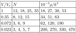
TABLE I. Simulated atom numbers for each trap volume and the corresponding peak atom densities.
V /Ve N 10−3ρ/k3
1 12, 18, 25, 35 18, 27, 38, 53 0.35 8, 12, 15 34, 51, 63 0.072 3, 6, 9 62, 120, 190 0.023 3, 4, 5, 7 200, 270, 330, 470
the order of averaging had a negligible effect on the pop-ulation decay (much less than 1%).
The quantitative comparison between the simulated and experimental results is made via the saturation parameter, defined as s = Ω2
R/2Γ
2, with Ω
R the
Rabi frequency and Γ = 2π×3.03 MHz HWHM. In Eqs. (8) above, the Rabi frequency is given by ΩR =
(ξ√2/D)ˆe∗1·D+F(Xj)
. The experimental value of s is obtained as s = (1/12)I/I
s, with Is = 1.67 mW/cm2.
The factor1/12 is the product of three factors: 1/2 from
projection ontoσ+polarization component;1/2from the
(squared) reduced dipole moment of theF = 2→F0 = 2 hyperfine component; 1/3 from the squared
Clebsch-Gordan coefficient of the|2,2i → |20,10itransition. Finally, in order to generate the results shown in the figures of the main section, we calculate in the simula-tions the remaining population in the initial state ρ11
as a function of time. This yields exponential decay rates (calculated from the initial population and from the t= 500/Γ results), or the pumping rates, each of which is represented by a single data point in Fig. 4(a) of the main text. The different data sets in Fig. 4 are obtained for different cloud volumes, resulting in the variation of both the atom density and optical thickness. Table I shows the simulated atom numbers for atom clouds whose volumes are smaller by the factor V /Ve than the experimental
value (the aspect ratios are the same in all cases).
NUMBER OF ATOMS CALCULATION
In this experiment we use absorption imaging in order to measure the optical thickness of the atomic clouds. The optical thickness is then converted to number of atoms per pixel. This conversion depends on the camera pixel size, the magnification, and the absorption cross sectionσ. Our camera’s pixel size and magnification are known (13µm and 13, respectively), butσshould be sim-ulated. For an imaging laser withσ+polarization driving
the|2,2i → |3,3itransitionσ0= 3λ2/2π. In our system,
however, the initial state is a distribution over the mF
order to find the effective cross section σeff (time
aver-aged over the imaging pulse) we solve the optical Bloch equations (OBE) for the 12 relevant states (5 Zeeman sublevels of theF = 2 ground state, and 7 for theF0= 3 excited state) using our experimental parameters (s1 and B = 5.4 G) with different initial conditions (initial distribution). We find that
σeff = (0.15±0.02)σ0. (9)
The error in σeff is due to the different initial
distribu-tions, and it is the main contribution to the error bars in number of atoms in the figures (the other source of error is shot-to-shot fluctuations). We would like to note that σeff includes a factor 0.5 to compensate the
retro-reflecting imaging scheme we use.
In order to improve our image quality and lower the noise in the image and the number of atoms we use two more algorithms: fringe removal and deconvolution. The fringe removal algorithm [5] takes an array of images of the imaging laser with no atomic cloud and generates a new image, which is a linear combination of these images, that minimizes the fringe visibility in the optical density image. This minimization is done in an area with no atoms, and the linear combination has different weights for each measurement. This algorithm deals with the main noise contribution that comes from fringes due to spurious reflections, which does not cancel well in the optical density image. It assumes that if these fringes will be canceled in the area near the atoms, this cancelation will be valid also in the area with atoms.
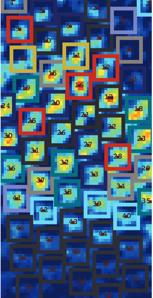
The second algorithm, the deconvolution, is performed because signal from one microtrap ‘leaks’ to neighboring sites. This leakage is a convolution of the ‘real’ number of atoms with a point-spread-function (PSF). Using a second order correlation matrixg(2) we confirm that the signal in each trap depends on its neighboring sites. We also find, using a fitting algorithm, a PSF that creates the same dependence of a site on it neighbors (the correlation matrix). The last step is to deconvolute our images with the fitted PSF. We would like to note that here we do not use the single pixels of the CCD. We rather sum a square around each microtrap [the square in Fig. 1] and use it as a ‘pixel’ for the deconvolution algorithm. The deconvoluted number of atoms is presented in figures 2 and 3 in the main text of the paper.
MICROTRAPS GROUPS
The analysis in this work was not done on a single cloud level, but rather on groups of clouds. This was done in order to reduce noise. The grouping was done based on the initial number of atoms in each site, which is averaged over 26 images. Figure 1 shows the area where we perform our analysis, and the individual microtraps. The pumping time is zero in the figure, and it shows
1
2
3
4
5
6
7
8
9
10
11
12
13
14
15
16
17
18
19
20
21
22
23
24
25
26
27
28
29
30
31
32
33
34
35
36
37
38
39
40
41
42
43
44
45
46
47
48
49
50
51
52
53
[image:4.612.316.564.55.537.2]54
55
FIG. 1. The analysis area. Each microtrap center is marked with a red dot and a site index. The squares around the mi-crotraps represent the area where we count the atoms, and the colors indicate the groups (see Table II). Traps that appear to be cut still use a full-size square to count the number of atoms by counting the relevant area outside the image shown here.
TABLE II. Grouping of microtraps based on initial number of atoms.
site index N0
group 1 1, 39, 40, 42 33±5 group 2 3, 41 58±8 group 3 4, 8, 15, 29, 34, 37 84±11 group 4 18, 19, 23, 32, 35, 36, 38 103±14 group 5 5, 6, 20, 24, 27, 30 131±18 group 6 10, 13, 33 157±21 group 7 17, 21, 22, 26, 31 181±24 group 8 9, 12, 16, 25, 28 204±27 group 9 11, 14 232±31
[1] Juha Javanainen, Janne Ruostekoski, Bjarne Vestergaard, and Matthew R. Francis, “One-dimensional modelling of light propagation in dense and degenerate samples,” Phys. Rev. A59, 649–666 (1999).
[2] Mark D. Lee, Stewart D. Jenkins, and Janne Ruostekoski, “Stochastic methods for light propagation and recurrent scattering in saturated and nonsaturated atomic ensem-bles,” Phys. Rev. A93, 063803 (2016).
[3] John David Jackson, Classical Electrodynamics, 3rd ed. (Wiley, New York, 1999).
[4] Stewart D. Jenkins and Janne Ruostekoski, “Controlled manipulation of light by cooperative response of atoms in an optical lattice,” Phys. Rev. A86, 031602 (2012). [5] C. F. Ockeloen, A. F. Tauschinsky, R. J. C. Spreeuw, and