Single Image Super Resolution Using Multi Scale Deep Encoder Decoder with Phase Congruency Edge Map Guidance

Single Image Super-Resolution Using Multi-Scale Deep

Encoder-Decoder with Phase Congruency Edge Map

Guidance

Heng Liua, Zilin Fua, Jungong Hanb, Ling Shaoc, Shudong Houa, Yuezhong Chua

a_{Anhui University of Technology, China, 243032} b_{Lancaster University, U.K., LA1 4YW} c_{University of East Anglia, U.K., NR4 7TJ}

Abstract

This paper presents an end-to-end multi-scale deep encoder (convolution) and decoder (deconvolution) network for single image super-resolution (SISR) guided by phase congruency (PC) edge map. Our system starts by a single scale symmetrical encoder-decoder structure for SISR, which is extended to a multi-scale model by integrating wavelet multi-resolution analysis into our network. The new multi-scale deep learning system allows the low resolution (LR) input and its PC edge map to be combined so as to precisely predict the multi-scale super-resolved edge details with the guidance of the high-resolution (HR) PC edge map. In this way, the proposed deep model takes both the reconstruction of image pixels’ intensities and the recovery of multi-scale edge details into consideration under the same framework. We evaluate the proposed model on benchmark datasets of different data scenarios, such as Set14 and BSD100 natural images, Middlebury and New Tsukuba -depth images. The evaluations based on both PSNR and visual perception reveal that the proposed model is superior to the state-of-the-art methods.

Keywords:

1. Introduction

SISR usually refers to reconstructing or recovering an HR image from an LR image without losing high frequency details or reducing the image quality, where the LR image is usually undergone a degradation process, such as geometric deformation, motion blurring and down sampling. Super-resolving an LR image is basically an inverse process of the degradation model, with the goal to recover the missing high-frequency details in the original HR image, such as edges and textures. Obviously, the solution of such recovery is very ambiguous because there are many HR images that can produce the same LR image. Therefore, SISR is a highly ill-posed problem due to its non-unique solution.

In general, SISR can be implemented by three means, namely, the inter-polation based methods, the reconstruction based methods and the learning based methods [41, 42, 3, 48, 47]. The simple and fast SR methods em-ploy different discrete interpolations, such as linear, bilinear and bi-cubic interpolations, all of which rely on the smoothness assumptions. However, the smoothness assumption will result in jaggy and ringing effects due to the discontinuities in images. Reconstruction based SR methods, especially maximum a posteriori (MAP), actually model the image degradation process, which mainly focuses on how to get the forward observation model and how to achieve SR through the degradation model. In general, both interpolation and reconstruction based methods merely process the image signal at the pixel level. On the contrary, learning based methods, especially dictionary learning or sparse representation based ones [41, 42], pay more attention to the understanding of the image content and structure, for which the prior knowledge in relation to image data imposes the constraints on the data for a better reconstruction. Given the training dataset, learning based SISR methods intends to learn an implicit mapping function between the low reso-lution (LR) images and the high resoreso-lution (HR) images, which have received considerable attention in the past few years.

for specific tasks. In addition, unlike traditional learning based methods, CNN based methods are end-to-end and can be more capable of directly ap-proximating mapping function between LR images and HR images, which can integrate intermedia processing into one pipeline handily. The seminal work of SISR based on convolutional neural network (SRCNN) is first pro-posed by Dong et al. [4], where an implicit LR to HR mapping is acquired via building a three-layer convolutional network and superior performance has been achieved. In such a model, image patch extraction, representation, non-linear mapping and image reconstruction, are sequentially implemented, which tend to simulate the processing procedure of sparse coding to generate HR images. Without considering the image prior, SRCNN model becomes a generic framework for image super resolution due to its lightweight struc-ture and the end-to-end style. However, recent works [37, 6, 15] acknowledge that the deeper and more complex networks can lead to more superior SR performance, which significantly raises the difficulty of network training. In addition, the research works in [21, 43, 38] argue that introducing image edge priors will either accelerate the training convergence [21] or help improve the reconstruction quality [43, 38]. Nevertheless, issues such as what type of image edge priors suits better and what deep convolution network structure is appropriate to this task are not fully addressed in existing CNNs based works. Thus, the exploration of constructing a deeper and more complex network with favorable image edge priors integration needs to be carried out in depth.

(a) SRCNN-L [5] (b) MSDEPC (Proposed)

Figure 1: The edges in the super-resolved image produced by the proposed MSDEPC model (right) are much sharper than the ones produced by SRCNN-L [5] (left) (4× down-sampling).

layers, FCN is all composed of convolution and deconvolution operations, which are usually named as encoder and decoder, respectively. However, in the above FCNs, convolution is always followed by pooling while decon-volution is followed by un-pooling, thus directly applying FCNs for image restoration tasks may give rise to the loss of the image details. Moreover, most existing FCN works only consider the single scale convolution pipeline, which fails to take full use of multiple range context and image details for SISR. It should be pointed out that in all of the followings, without special statement, the items of encoder and decoder always refer to the operations of convolution and deconvolution.

In this work, for CNN based image SR, we want to investigate whether all kinds of image edge features are suitable and helpful, and how to construct an opportune deep model with the favorable of edge details. Considering the fact that multi-scale image contextual information is essential for the recon-struction of high-frequency image details, based on the network simulation of discrete wavelet multi-resolution analysis, we propose a multi-scale deep encoder-decoder structure for SISR. More specifically, we construct a three-scale encoder-decoder deeper network by cascading three convolution and deconvolution layers with varying length sizes. At each scale, deep encoder-decoder does not involve any pooling and un-pooling operations in order to avoid image details leaking during the image recovering. Then, motivated by the observation that phase congruency (PC) edge map [17], a kind of structural edge features of an image, is invariant against different scales sub-sampling, we manage to introduce the phase congruency edge map to guide the prediction of the edge features in our multi-scale model. By doing so, the proposed multi-scale deep SR model becomes capable of recovering the edge details alongside reconstructing the image intensities at different scales, in which the edge loss and the pixels’ value loss are combined to jointly supervise the training. An example of a super-resolved image through the proposed model from 4× down-sampling is illustrated and compared to SRCNN-L [5] in Fig. 1. Our proposed SISR deep model (abbreviated as MSDEPC) is illustrated in Fig. 2.

In summary, the contributions of our work are three-fold:

LR Image LR Edge HR Image HR Edge 32 32

32 32 32 32

32 64

32 32

Ă

64 64 64 32

Ă Edge Loss Image Loss Total Loss Conv+BN+ReLU Deconv+BN+ReLU 3 1 1 1 + + + 3 ¨ 2

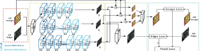
Figure 2: The proposed MSDEPC model: joint input of LR image and edge (red), multi-scale encoder-decoder learning (yellow), multi-multi-scale HR image and edge prediction (green), and the total loss (blue).

to generate the final reconstructed image.

•We integrate the PC edge prior into the deep network and balance the image intensity loss and the edge loss to jointly supervise the training. The comparisons and the experimental results show that the PC edge map is more suitable for SISR, compared to other types of edges, e.g., Canny edges and Sobel edges, in terms of the reconstruction quality.

•We verify and evaluate the proposed model on widely recognized public datasets, and also on completely different data from training images, e.g., depth images. We also compare the variants of our model and discuss the impact when taking different local structures of the network, which will be constructive and helpful for future SISR research.

The rest of this paper is organized as follows. In Section 2, the related works for SISR are reviewed in detail. In Section 3, the architecture and the constructing principle of the proposed deep model are described. Exper-imental results and discussions are provided in Section 4. Finally, Section 5 makes a brief conclusion and outlines the future work.

2. Related Work

2.1. Image Priors based Super-Resolution

As known, for image recovery tasks, image priors play an important role in regularizing the optimization process or imposing a constraint for a fast solution. So far, some image priors have been successfully applied for SISR, such as sparse prior [41, 42], exemplar prior [35, 46], and self-similarity prior [11, 49].

to be the same. Based on exemplar prior, Timofe et al. [35] proposed an anchored neighbourhood regression based approach, where the anchors refer to the learned dictionary atoms. Alternatively, Zhang et al. [46] utilized a mixture of experts (MoE) method to jointly learn the feature space partition and local regression models. Some recent studies in [11, 49] reveal that local image structure tends to occur within and across different image scales. Due to such self-similarity prior, image SR can be solved by using self-similar examples instead of the external data. On top of it, the internal patch search space of self-similarity methods can even be expandable if allowing geometric variations [11]. In addition, Gu et al. [6] regarded sparse prior based image SR as a filtering process. To address the inconsistency problem of pixels in the overlapped blocks, they raised a convolutional sparse coding based SR. However, this method, especially the training part, is rather expensive in the sense that three groups of parameters that need to be learned: LR filters, mapping functions and HR filters.

,some image priors have been recently introduced into the CNNs for SISR [37, 21], which will be elaborated below.

2.2. CNN based Image Super-Resolution

Benefiting from the powerful non-linear mapping, CNN based image SR, including the pioneer SRCNN [5, 4] and the very recent works [8, 7, 28], can improve the performance dramatically compared with the traditional meth-ods. One main weak of SRCNN is that the model actually is not deep enough and is trained without the prior knowledge considered, thereby leading to a very slow convergence speed. In [37], Wang et al. presented a compositional model combining sparse prior and a deep network, which demonstrates an efficient training/performance trade-off for SISR. Considering that directly training an SRCNN model takes too long to converge, Liang et al. [21] intro-duced Sobel edge detection so as to capture gradient information to accelerate the training convergence. In fact, the method does reduce the training time but the resultant reconstruction enhancement is limited. Again exploiting Sobel edge features, Yang et al. [43] described a recurrent residual learning method for SISR. However, in principle, Sobel edge features only acquire image magnitude step-jump discontinuities in both horizontal and vertical directions, but cannot preserve accurate and stable image edge details, espe-cially when applying sub-samplings at different scales.

can usually lead to a remarkable performance improvement. For example, Kim et al. [15] take twenty convolution layers with residual connected to construct SR network which accomplishes a significant improvement in SR reconstruction accuracy. Aiming to improve SISR, Ledig et al. [18] proposed to utilize a novel network structure - generative adversarial network (SR-GAN) to produce photo-realistic SR images. The SRGAN network consists of two distinct sub-networks and adopts an extended version of the percep-tion loss [14] for training, being defined based on the feature maps from the VGG network [34]. In spite of its surprisingly good performance, the latest evidence [27] suggests that the generated super-resolved image will be likely to contain some checkerboard artifacts. Moreover, in an effort to achieve real time SISR, Shi et al. [33] claim that directly learning upscaling filters through a network can improve the reconstruction performance both in accu-racy and speed. Actually, the proposed sub-pixel convolution layer is almost equivalent to the deconvolution layer but it requires more convolution filters to produce enough feature maps.

2.3. Deep Encoder and Decoder

ĂĂ

Conv Conv Deconv Deconv

LR Image

HR Image

Encoder Decoder

Conv+ReLU

Deconv+ReLU

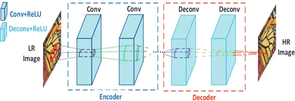
Figure 3: Single scale deep symmetrical encoder-decoder: the network only consists of convolutional and deconvolutional layers; PReLU layer follows after convolution or decon-volution operation.

3. Multi-scale Deep Encoder-Decoder Learning for Image SR

3.1. Design Basis for Multi-scale Encoder-Decoder

Designing a multi-scale deep encoder-decoder gains two main benefits: 1) multi-scale features can be easily extracted from the input image by multiple scales encoders and the SR image under different scales can be reconstructed through different scales decoders; 2) it is an end-to-end system, implying that it is convenient to adjust the network itself and observe the effects. However, due to the absence of previous references or reports, how to design a multi-scale encoder-decoder network for SISR becomes a new challenge. Fortunately, since SISR can be treated as a signal reconstruction task, we may take wavelet analysis [24], a well-known method for signal decompo-sition and reconstruction, to guide the network construction of multi-scale deep encoder-decoder. Actually, in this work, we adopt the network simula-tion strategy and implement the multi-scale analysis and reconstrucsimula-tion by the corresponding network operations, such as convolution, deconvolution, concation and summation.

Based on the wavelet multi-resolution analysis (MRA) [24], for an image

f(x) in L2 _{space R, it can be represented as:}

f(x) =

N

X

k∈Z

aj0

kφ

j0 k(x) +

J

X

j=j0

X

k

bj_kψ_kj(x), (1)

where j is the scale varying from j0 to J, k is the index of basis function,

and {aj0 k}, {b

j

k} are coefficients attached to the approximation (scale)

(see Eq. (1)): the approximation (the first item, low frequency component) and the details (the second item, high frequency components). That is if varying the scale j from zero to certain scale, f(x) can be represented as the weighted summation of a series of components or (sub-bands) at different scales, which contains a low frequency approximation and several or numer-able high frequency details. From deep learning point of view, Eq. (1) on the whole may be treated as the combination of deconvolution (reconstruction) operations at multiple scales. In the equation, the approximation coefficients

aj_k and the detail coefficients bj_k are the projections of imagef(x) to different approximation subspaces or detail subspaces at different scale j. Actually,

aj_k and bj_k can be calculated as:

aj_k =hf(x), φj_k(x)i=X

i

pj_ikfi

bj_k =hf(x), ψ_kj(x)i=X

i

qj_ikfi

(2)

Here, assuming the image f(x) is discretized as f = {f1, f2,· · · , fi,· · · },

the scale function φj_k is relaxed to {pj_1k, pj_2k,· · · , pj_ik,· · · }, and the wavelet function ψ_kj is relaxed to {qj_1k, q₂j_k,· · · , q_ikj ,· · · }. According to convolutional hierarchical feature learning in [44], if regarding the weights pj_ik and q_ikj as the kernels of the convolution layers at certain scale j and treating the inner projection as the procedure of feature encoding, Eq. (2) will be realized by one scale encoding (convolution) on the image f(x). Accordingly, aj_k and

bj_k will become the feature map outputs of these encoders at certain scale. Naturally, if also introducing the decoder’s weights ˜pj_ik and ˜q_ikj as the kernels of the deconvolution layers, then based on Eq.(1) the reconstructed image

˜

f(x) can be obtained by multi-scale decoding (deconvolution) as:

˜

f(x) = X

j

X

k

X

i

˜

pj_ikaj_k+X

j

X

k

X

i

˜

q_ikj bj_k (3)

3.2. Multi-scale Encoder-Decoder Learning

Obviously, by cascading the convolution and deconvolution with different lengths, the encoding and decoding of imagef(x) can be carried out continu-ously from coarse scale (short stream) to fine scale (long stream). Assuming the network stream at each scale, denoted as ˜fj, represents an

approxima-tion of f(x). Thus, according to Eq. (3), if we take a summation function

s adding up all encoder-decoder streams, the multi-scale encoder-decoder reconstruction ˜f(x) can be easily acquired as:

˜

f(x) =s( ˜f1,f˜2,· · · ,f˜j,· · ·) (4)

Therefore, through such multi-scale expansion, the primary content and the details of an HR image can be gradually recovered. Particularly, if we regard the LR image also as an approximation of HR image f and input it to the network, the super-resolved image ˜f can be generated from the multi-scale encoder-decoder structure by replacing the summation function s in Eq. (4) with the network summation operation.

The optimization target of multi-scale encoder-decoder learning can be regarded as:

˜

f = arg min

f (

X

j

F_ja(y,Θ_j)−f_ja 2 2+ X j

F_jb(y,Θ_j)−f_jb

2

2), (5)

wheref and yrepresent the HR image and the corresponding LR image, and

F(·) denotes the network reconstruction function. Θ is the learned parameter of the network and symbols j, a, b indicate a specific scale, a low frequency approximation component and a high frequency component, separately. By taking into account the components of different scales simultaneously, multi-scale encoder-decoder learning will overcome the deficiency of only consider-ing the similarity ofL2 _{−norm energy (mainly concentrated in low frequency}

components) whilst ignoring the recovery of the structural details (in high frequency components).

Given a set of LR and HR image pairs {fi, yi}Ni=1 and assuming the

ap-proximation and detail components of HR image fi at multiple scales can

be obtained, then according to Eq. (5), the loss function of the proposed multi-scale encoder and decoder can be denoted as:

Loss=X

j λj N X i=1

F_ja(y_i,Θ_j)−f_j,ia 2 +X j βj N X i=1

F_jb(y_i,Θ_j)−f_j,ib

2

where λ and β are regulation coefficients for every loss term. All other symbols are the same as those in Eq. (5). However, to facilitate training and simplify regulation, the loss function can be relaxed to Eq. (8) by: 1)

synthesizing multiple components of different scales to two components (low frequency approximation and high frequency detail, Eq. (7)); 2) replacing the approximation component with the input LR image and specifying the detail component as one special type of it - PC edge map.

Loss(Θ)≈λ

N

X

i=1

kFa_(y

i,Θ)−fiak 2 +β N X i=1

Fb(yi,Θ)−fib

2

, (7)

Loss(Θ)≈

N

X

i=1

kF(yi,Θ)−fik 2

+η

N

X

i=1

kF(Lei,Θ)−Heik 2

, (8)

where η can be regarded as a trade-off, regulating the reconstruction focus of the energy approximation term (the first term, low frequency component) and the edge similarity term (the second term, high frequency details ). More discussions on the effect of each term in the loss function can be referred to the first part of Section 4.4. Lei and Hei denote the ith extracted LR and

HR edges using the PC edge map operator, separately. F(Lei,Θ) represents

the prediction of the edge map of the super-resolved image.

3.3. Edge Map Guidance

If the observed LR imageyis regarded as the low-frequency component of the HR image, then the high frequency components are just the details of the image, such as textures, edges or corners. In other words, recovering image details becomes the most pivotal requirement for SISR. This motivates us to use the image details to guide SR image reconstruction rather than using the pixels’ intensity values only. With respect to the proposed deep model, the guidance provided by image details is composed of two aspects: taking the HR image details for network supervision and integrating the corresponding LR image details with itself as the network input.

(a) Original (b) Canny edge (c) Sobel edge (d) PC edge map

(e) Canny edge of 3×DS

(f) Sobel edge of 3×DS

(g) PC edge map of 2×DS

(h) PC edge map of 3×DS

Figure 4: PC edge map vs. Canny or Sobel edge when down-sampling (DS) with different scales.

the problem that the edge location will not be consistent or will even be completely different.

In view of this, Kovesi in [16] argued that the Fourier components of a signal are all in phase at the point of the step in the square wave, and at the peaks and troughs of the triangular wave. This property, named phase congruency (PC), is stable over scale and intensity, which can be measured as the following if at a location x:

P C(x) = W(x) inf (_P |E(x)| −T)

A(x) +ε , (9)

where A(x) is the amplitude, W(x) is a weighting function for frequency spread, E(x) is local energy, ε is small constant to avoid division by 0, and

network to improve SISR by jointly supervising the training. More details concerning the PC edge map as well as its extraction may be found in [17]. The comparisons between the PC edge map and the traditional edge features are illustrated in Fig. 4.

We can take the stability and the consistency of the features across dif-ferent scales to measure the performance difference of the edge feature ex-traction methods. As can be seen from Fig. 4, the traditional edge features (Canny or Sobel) of 3×3 down-sampling are obviously distinct from the orig-inal traditional edge features (see (e) to (b) and (f) to (c)). Compared to the original edge features, they lose many structural details and introduce some artifacts. In other words, the traditional edge features are not robust when image down-sampling occurs. Whereas PC edge maps across different scales are basically consistent and never produce any artifacts (see (h) to (g) and (d)). Therefore, the PC edge map is superior to the traditional edge features in terms of the stability and consistency at different scales.

3.4. Model Architecture

The architecture of the proposed model can be divided into four algo-rithmic steps (see Fig. 2). The specific configurations of all convolution and deconvolution layers can be found in Table 1.

In the first step, two components are integrated as input and fed into the network, that is, an LR image with its corresponding PC edge map. This can also be interpreted as we integrate the two components to learn.

In the second step, the joint input is sent to a multi-scale network to fuse learned multi-scale features. In our model, we use a three-scale encoder-decoder symmetrical network in order to obtain better image reconstruction performance. Next, the multiple streams are connected by side outputs sim-ilar to the connections in works [39, 32]. Here, relatively fewer filters (e.g. 32) and smaller kernel sizes (e.g. 3×3) are adopted in the convolutional layers because we want to reduce the computation load of the network and we believe that connecting convolution layers through cascading can simulate any sizes of receptive field [34].

(see three direct links from the input to the summation units) to get three reconstructed images at different scales. Furthermore, the reconstructed ones are also integrated to get the final super-resolved image.

At last, in the fourth part, the image intensity loss and the edge map loss are combined with the weight η for the supervised training.

In order to alleviate the difficulty in training convergence, PReLU acti-vation function [10] with batch normalization layer [12] (BN) is added into our architecture. In practice, we find that such two tricks can also improve the reconstruction quality.

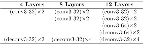
Table 1: The configuration of three scales encoder-decoder streams (4 layers, 8 layers and 12 layers): conv3 and deconv3 stand for convolution and deconvolution layers with kernel size 3×3 andstride= 1; 32 and 64 are the numbers of filters.

4 Layers 8 Layers 12 Layers

(conv3-32)×2 (conv3-32)×2 (conv3-32)×2 (conv3-32)×2 (conv3-32)×2 (conv3-64)×2 (deconv3-64)×2 (deconv3-32)×2 (deconv3-32)×4 (deconv3-32)×4

3.5. Computation Complexity

From the computation point of view, a deep learning model, especially a convolutional neural network, needs to perform forward computation (mak-ing the input convolution and the output estimation) and backward propa-gation (computing the gradient and making the gradient convolution). Ob-viously, the computation of the whole deep network depends on the tation of each layer. The most complex (the most time-consuming) compu-tation of each layer is the convolution, the time complexity of which domi-nantly depends on the parameters of the layer and the size of the input data to it. Since the proposed multi-scale deep encoder-decoder is a kind of fully convolutional network model, its computational complexity can actually be deduced from the complexity of a single convolution layer.

For any convolution layer, assuming the number of input channel is Cin,

the number of output channel is Cout, the size of feature map (output) is

M, and the size of convolution kernel is K, then the time complexity of the convolution layer is:

Thus, for the proposed multi-scale encoder-decoder, assuming there are S

scales, the total number of all convolution layers in each scale network (the depth) is Ds, the numbers of the input channel and the output channel of

the lth _{convolution layer in each scale branch are C}

l−1 and Cl, respectively,

then the time complexity of the multi-scale model is:

T ime ∼O(

S

X

s=1 Ds

X

l=1

M_l2·K2

l·Cl−1·Cl) (11)

The space complexity of the proposed method depends on the parameters of the model, which can be formulated as:

Space∼O(

S

X

s=1 Ds

X

l=1

K_l2·Cl−1·Cl) (12)

4. Experiments and Analysis

4.1. Datasets and Evaluation Measures

We perform experiments and compare the algorithm performance on three widely acknowledged test data sets: Set5 [2], Set14 [45] and BSD100 [25]. For a fair comparison, our model is firstly trained with 91 images [35] which were extensively used in the previous works. Then, the entire framework is re-trained from scratch with 50,000 images collected from ImageNet [30] similar to [5, 18, 33]. Regarding the quality measurement of the reconstructed images, despite some recent no-reference metric works, such as [23], we still use the well-known PSNR [dB] and SSIM [36] metrics. One specific network is trained per super-resolution factor.

4.2. Training Details

low-resolution pairs are acquired by imposing the bi-cubic interpolation twice (same to the works [4, 5]) on the ground truth, and the PC edge pairs are extracted with multiple scales by Log-Gabor filter banks at the same time.

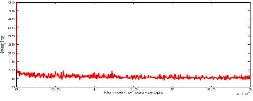
In our framework, we follow the suggestions from He et al. [10, 9] to initialize the weights. Whilst training the framework, we initially set the learning rate to 0.01 and enable gradient clipping (GC). In our experiments, we clip the gradient to 10 first, and then change it to 1 when the loss value plateaus. Momentum and weight decay parameters are set to 0.9 and 0.0001, respectively. The edge loss coefficient η is a hyper parameter which can be determined by cross-validation with multiple folds or by the random search approach [1]. In practice, we set it to be 1 at the beginning and then man-ually adjusted it to 0.1, emphasizing the impact of image intensity recon-struction once the gradient becomes relatively small. The whole deep net-work training is implemented using the Caffe package [13] with one TITANT X GPU. The training loss convergence curve of 4× down-scaling SISR is shown in Fig. 5. The source code and the model can be downloaded at https://github.com/hengliusky/Muti-scale SuperResolution. As for the Im-ageNet dataset training, all settings are the same as the 91-image dataset.

0 0.5 1 1.5 2 2.5 3

x 105

0 5 10 15 20 25 30 35 40 45 50

Number of backprops

Training Loss

Figure 5: 4×down-scaling training convergence curve.

4.3. Variant Models

As mentioned above, our system consists of four parts. Modifying/changing any of them with other structure will bring about the variants of our model. A special variant is to replace the multiple scales parts (yellow and green parts in Fig. 2) with single scale structure while maintaining PC edge map. We name such special varaint as MSDEPC-V1. In addition, based on MS-DEPC, other trivial variants include substituting the PC edge map with

overall structure unchanged. We will train these variant models and compare their reconstruction performance in the following to illustrate whether they are suitable or not for our multi-scale encoder-decoder based SISR.

4.4. Analysis and Comparisons

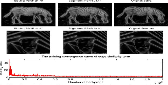
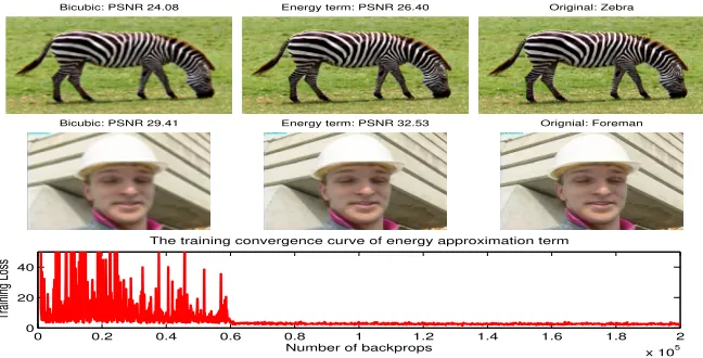
Impact Analysis of The Terms in Loss Function. The terms in loss function, see Eq.8, are the energy approximation term (the first term) and the edge similarity term (the second term), respectively. To clarify the impact of each of these two terms for SISR, we separately utilize each term to supervise the network learning and then evaluate the corresponding reconstruction results. Here, all training settings and parameters are exactly the same as those of original 4× SR model. The convergence curve and some reconstruction results of the edge similarity supervision are illustrated in Fig. 6 whereas the corresponding ones of the image energy approximation term are shown in Fig. 7.

0 0.2 0.4 0.6 0.8 1 1.2 1.4 1.6 1.8 2

x 105 0

20 40

Number of backprops

Training Loss

The training convergence curve of edge similarity term

Bicubic: PSNR 21.70 Edge term: PSNR 24.17 Original: Zebra

Bicubic: PSNR 25.57 Edge term: PSNR 28.50 Orignial: Foreman

Figure 6: The effect of edge similarity supervision: 4×down-scaling training convergence curve (the bottom row); some reconstructed edges (the middle column of upper two rows).

0 0.2 0.4 0.6 0.8 1 1.2 1.4 1.6 1.8 2

x 105

0 20 40

Number of backprops

Training Loss

The training convergence curve of energy approximation term Bicubic: PSNR 24.08 Energy term: PSNR 26.40 Original: Zebra

Bicubic: PSNR 29.41 Energy term: PSNR 32.53 Orignial: Foreman

Figure 7: The effect of image energy approximation learning: 4×down-scaling training convergence curve (the bottom row); some reconstructed images (the middle column of upper two rows).

Guidance Effectiveness of PC Edge Map. In order to investigate the guidance effectiveness of PC edge map for SISR, in Table 2, we compare the recon-struction performance of those variants which take the PC map [16] or Canny edge features to replace the original PC edge with no structure changed. For ease of explanation, such two variants are denoted as MSDEPC-V2 and MSDEPC-V3, respectively. Meanwhile, MSDEPC-V1 mentioned above is also included in Table 2. Additionally, for a more clear understanding of the role of the PC edge map input, in the table we also list the performance of the deep encoder-decoder symmetrical network (abbreviated as DEDSN), which has no any edge input. The structure of DEDSN is shown in Fig. 3. Here, for convenience only the single scale is considered. Note that the configurations and the parameters of DEDSN are exactly the same as that of MSDEVP-1, except that it only uses LR images as input.

As a result, we have in total five deep frameworks involved in the compar-ison, alongside the baseline model SRCNN. Testing those variants effectively verifies the proposed contributions, which are the multi-scale deep encoder-decoder learning framework and the involvement of the PC edge map in our model training. It should be noted that in such comparisons all variants are trained based on the 91-image dataset, retaining the same settings of the original MSDEPC model.

Table 2: The SR performance comparisons of the variants in terms of the averaged PSNR (dB) and SSIM [36] (upper and lower numbers, respectively). Best results are indicated in Bold.

Dataset Set5 Set14 BSD100

×3 ×4 ×2 ×3 ×2 ×4

SRCNN[4] 32.37 30.03 32.18 29.00 31.11 26.70

0.9033 0.8530 0.9017 0.8145 0.8835 0.7078

MSDEPC-V1 32.90 30.78 32.74 29.34 31.58 26.90

0.9125 0.8745 0.9088 0.8196 0.8920 0.7135

MSDEPC-V2 32.71 30.45 32.47 29.05 31.29 26.73

0.9095 0.8696 0.9040 0.8098 0.8851 0.7074

MSDEPC-V3 31.47 29.67 31.94 28.70 30.88 26.45

0.8904 0.8506 0.8981 0.8066 0.8807 0.7011

DEDSN 32.75 30.53 32.42 29.10 31.41 26.78

0.9105 0.8675 0.9031 0.8094 0.8869 0.7090

MSDEPC 33.37 31.05 32.94 29.62 31.64 27.10 0.9184 0.8797 0.9111 0.8279 0.8961 0.7193

model to improve the super-resolution quality. This conclusion can also be confirmed even if we compare DEDSN and MSDEPC-V1 separately. We will find that the former (without edge input) is much worse than the latter (with edge input) in terms of the performance. However, not all types of edge features are suitable for doing so, at least for our multi-scale model. For example, Canny edge features, introduced in the variant model - MSDEPC-V3 is inappropriate for SISR in view of the lower PSNR and SSIM.

The fact that the framework guided by PC map (MSDEPC-V2) performs worse, at every scale sub-sampling, than the framework using PC edge map (MSDEPC) implies that, for the SISR task, incorporating more types of im-age features actually cannot guarantee a better reconstruction performance. It is clear that MSDEPC and MSDEPC-V1 both integrating PC edge maps, demonstrate much stronger performance than others. This observation might indicate that PC edge map is indeed a kind of effective edge features for im-proving SISR.

Table 3: Convergence speed comparisons: with or without BN and GC.

Training epochs MSDEPC MSDEPC-V1 MSDEPC-V2 MSDEPC-V3

×2 ×4 ×2 ×4 ×2 ×4 ×2 ×4

With BN and GC 913 85 796 75 131 62 527 160

W/O BN and GC 1097 167 821 143 201 75 626 234

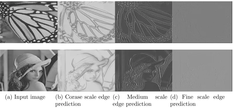
Multiple Scales Edge Prediction. To show the ability of the proposed multi-scale model, the predicted three multi-scales’ edge maps of two test images during a training session are shown in Fig. 8. From the figure, it is clear that training the model can capture image edge details at different scales. The shortest encoder-decoder stream (4 layers), which corresponds to coarse scale, can capture all massive edges; the middle length encoder-decoder stream (8 layers), corresponding to the medium scale, can strengthen the meso-scale edges; while the longest cascading one (12 layers), corresponding to the fine scale, can acquire the smallest edge details. Additionally, it is also shown the more layers involved in the network, the finer the scale will be.

(a) Input image (b) Corase scale edge prediction

(c) Medium scale

edge prediction

(d) Fine scale edge prediction

Figure 8: Multi-scale edge prediction extracted from a network training session. From left to right: original image, coarse scale (4 layers) edge prediction, medium scale (8 layers) edge prediction and fine scale (12 layers) one.

SISR, for fairness, we do not make comparisons with them. Depending on the training datasets, the comparisons are divided into two groups: Table 4 lists the methods trained by 91-images while Table 5 shows those trained by ImageNet or others. According to the results in Table 4 and Table 5, the proposed MSDEPC model can obtain the best performance in most cases, and only performs a little worse at several particular spots than the VDSR [15], which is the best published algorithm. From the algorithm perspective, the reason why VDSR is occasionally better than us might be the deeper net-work (20 vs 12) with more filters in each layer (64 vs 32), which inspires us to deepen our multi-scale architecture and make more dense filters in future work.

The running time comparisons (three times average) of 4× SISR for 512×512 input between the proposed model and the other CNN-based meth-ods are shown in Table 6. From the table, it is clear that if using GPU to perform SISR, the time-consuming difference between the proposed method and the other methods is almost smoothed out. But the gap does exist if CPU is used. At such time, the proposed method is about five times faster than VDSR and only a little slower than SRCNN-L (only contains three layers). The visual qualities of the super-resolved images generated by our model and also the other competing models based on different test datasets are illustrated in Fig. 9 and Fig. 10.

Table 4: The mean PSNR (dB) (left numbers) and SSIM (right numbers) for different methods trained with 91-images. Best results are indicated in Bold.

Dataset

Set5 Set14 BSD100

×2 ×3 ×4 ×2 ×3 ×4 ×2 ×3 ×4

Bicubic 33.66\0.9299 30.39\0.8682 28.42\0.8104 30.24\0.8687 27.55\0.7736 26.00\0.7019 29.56\0.8431 27.21\0.7385 25.96\0.6675

SRCNN[4] 36.34\0.9521 32.37\0.9033 30.03\0.8530 32.18\0.9017 29.00\0.8145 27.20\0.7413 31.11\0.8835 28.20\0.7794 26.70\0.7078

ESPCN[33] −\− 32.55\− −\− −\− 29.08\− −\− −\− 28.26\− −\−

MSDEPC 37.39\0.9576 33.37\0.9184 31.05\0.8797 32.94\0.9111 29.62\0.8279 27.79\0.7581 31.64\0.8961 28.58\0.7918 27.10\0.7193

(a) Bicubic: 24.08 (b) SRCNN-L: 26.09 (c) MSDEPC: 26.54 (d) Original: Zebra

(a) Bicubic: 27.55 (b) SRCNN-L: 30.22 (c) MSDEPC: 30.83 (d) Orignal: Monarch

(a) Bicubic: 29.41 (b) SRCNN-L: 32.24 (c) MSDEPC: 32.90 (d) Orignal: Monarch

(a) Bicubic: 21.98 (b) SRCNN-L: 24.80 (c) MSDEPC: 25.78 (d) Orignal: Monarch

(a) SRCNN-L: 21.53 (b) VDSR: 21.71 (c) MSDEPC: 21.82 (d) Original: 148026

(a) SRCNN-L: 33.01 (b) VDSR: 33.67 (c) MSDEPC: 33.78 (d) Orignal: 106024

(a) SRCNN-L: 24.80 (b) VDSR: 25.85 (c) MSDEPC: 25.93 (d) Original: 86000

(a) SRCNN-L: 26.36 db (b) VDSR: 26.61 db (c) MSDEPC: 26.67 db (d) Orignal: 19201

(a) Bicubic: 37.43 db (b) SRCNN-L: 40.84 db

(c) MSDEPC: 41.67 db (d) Orignal: Middlebury

(a) Bicubic: 27.43 db (b) SRCNN-L: 30.84 db

(c) MSDEPC: 31.59 db (d) Original: New Tsukuba

Table 5: The mean PSNR (dB) (left numbers) and SSIM (right numbers) for different methods trained with ImageNet or others. Best results are indicated in Bold.

Dataset

Set5 Set14 BSD100

×2 ×3 ×4 ×2 ×3 ×4 ×2 ×3 ×4

SRCNN-L[5] 36.66\0.9542 32.75\0.9090 30.49\0.8628 32.45\0.9027 29.30\0.8251 27.50\0.7513 31.36\0.8876 28.41\0.7853 26.90\0.7186

SelfExSR[11] 36.62\0.9548 32.66\0.9098 30.35\0.8607 32.31\0.9070 29.16\0.8209 27.30\0.7499 31.32\0.8835 28.33\0.7778 26.80\0.7120

ESPCN[33] −\− 33.13\− 30.90\− −\− 29.49\− 27.73\− −\− 28.54\− 27.06\−

VDSR[15] 37.53\0.9578 33.65\0.9210 31.33\0.8834 33.03\0.9124 29.75\0.8312 27.95\0.7671 31.90\0.8960 28.80\0.7970 27.24\0.7245

MSDEPC 37.54\0.9587 33.70\0.9225 31.41\0.8836 32.96\0.9117 29.78\0.8319 28.02\0.7679 31.92\0.8967 28.88\0.7974 27.30\0.7249

Table 6: Running time comparisons (Seconds; with one TITAN X).

Running time SRCNN-L VDSR MSDEPC

With GPU 0.188 0.245 0.241

Without GPU 11.417 74.053 15.269

5. Conclusion

In this work, by presenting a new MSDEPC model, we have demonstrated that multi-scale deep structure with appropriate edge details integration will significantly facilitate the task of SISR.

We explored the relationship between signal wavelet multi-scale analysis and multi-scale encoder-decoder learning networks, based on which we have constructed a three-scale encoder-decoder deep model for SISR. Moreover, we integrated the important image structural features − phase congruency edge into the multi-scale network to ensure the recovery of image structural edge details. Experimental comparisons showed that the proposed approach outperforms the state-of-the-art methods.

Future work will focus on two aspects. Directly learning upscaling-filters by introducing the deconvolution into each scale network is the near future task. Investigating the perception loss and fusing image classification task with super-resolution into current multi-scale learning architecture will be the long term target.

Acknowledgment

References

[1] Bergstra, J., Bengio, Y., 2012. Random search for hyper-parameter op-timization. Journal of Machine Learning Research 13 (Feb), 281–305.

[2] Bevilacqua, M., Roumy, A., Guillemot, C., Alberi-Morel, M. L., 2012. Low-complexity single-image super-resolution based on nonnegative neighbor embedding. In: Proc. British Machine Vision Conf. pp. 1–10.

[3] Choi, J.-S., Kim, M., 2017. Single image super-resolution using global regression based on multiple local linear mappings. IEEE Transactions on Image Processing 26 (3), 1300–1314.

[4] Dong, C., Loy, C. C., He, K., Tang, X., 2014. Learning a deep convolu-tional network for image super-resolution. In: Proc. Eur. Conf. Comput. Vis. pp. 184–199.

[5] Dong, C., Loy, C. C., He, K., Tang, X., 2016. Image super-resolution using deep convolutional networks. IEEE Trans. Pattern Anal. Mach. Intell. 38 (2), 295–307.

[6] Gu, S., Zuo, W., Xie, Q., Meng, D., Feng, X., Zhang, L., 2015. Convo-lutional sparse coding for image super-resolution. In: Proc. IEEE Int. Conf. Comput. Vis. Pattern Recognit. pp. 1823–1831.

[7] Han, W., Chang, S., Liu, D., Yu, M., Witbrock, M., Huang, T. S., 2018. Image super-resolution via dual-state recurrent networks. In: Proceed-ings of the IEEE Conference on Computer Vision and Pattern Recogni-tion. pp. 1654–1663.

[8] Haris, M., Shakhnarovich, G., Ukita, N., 2018. Deep back-projection networks for super-resolution. In: Proceedings of the IEEE Conference on Computer Vision and Pattern Recognition. pp. 1664–1673.

[9] He, K., Zhang, X., Ren, S., Sun, J., 2015. Deep residual learning for image recognition. arXiv preprint arXiv:1512.03385.

[11] Huang, J.-B., Singh, A., Ahuja, N., 2015. Single image super-resolution from transformed self-exemplars. In: Proc. IEEE Int. Conf. Comput. Vis. Pattern Recognit. pp. 5197–5206.

[12] Ioffe, S., Szegedy, C., 2015. Batch normalization: Accelerating deep network training by reducing internal covariate shift. arXiv preprint arXiv:1502.03167.

[13] Jia, Y., Shelhamer, E., Donahue, J., Karayev, S., Long, J., Girshick, R., Guadarrama, S., Darrell, T., 2014. Caffe: Convolutional architecture for fast feature embedding. In: Proc. ACM Int. Conf. Multimedia. pp. 675–678.

[14] Johnson, J., Alahi, A., Fei-Fei, L., 2016. Perceptual losses for real-time style transfer and super-resolution. In: Proc. Eur. Conf. Comput. Vis. pp. 694–711.

[15] Kim, J., Kwon Lee, J., Mu Lee, K., 2016. Accurate image super-resolution using very deep convolutional networks. In: Proc. IEEE Int. Conf. Comput. Vis. Pattern Recognit. pp. 1646–1654.

[16] Kovesi, P., 1999. Image features from phase congruency. J. Comput. Vis. Res. 1 (3), 1–26.

[17] Kovesi, P., 2003. Phase congruency detects corners and edges. In: Proc. Australian Pattern Recog. Soc. Conf.

[18] Ledig, C., Theis, L., Husz´ar, F., Caballero, J., Aitken, A., Tejani, A., Totz, J., Wang, Z., Shi, W., 2016. Photo-realistic single image super-resolution using a generative adversarial network. arXiv preprint arXiv:1609.04802.

[19] Li, Z., Tang, J., 2015. Weakly supervised deep metric learning for community-contributed image retrieval. IEEE Transactions on Multi-media 17 (11), 1989–1999.

[21] Liang, Y., Wang, J., Zhou, S., Gong, Y., Zheng, N., 2016. Incorporating image priors with deep convolutional neural networks for image super-resolution. Neurocomputing 194, 340–347.

[22] Long, J., Shelhamer, E., Darrell, T., 2015. Fully convolutional networks for semantic segmentation. In: Proc. IEEE Int. Conf. Comput. Vis. Pattern Recognit. pp. 3431–3440.

[23] Ma, C., Yang, C.-Y., Yang, X., Yang, M.-H., 2017. Learning a no-reference quality metric for single-image super-resolution. Computer Vi-sion and Image Understanding 158, 1–16.

[24] Mallat, S., 1999. A wavelet tour of signal processing. Academic press.

[25] Martin, D., Fowlkes, C., Tal, D., Malik, J., 2001. A database of human segmented natural images and its application to evaluating segmentation algorithms and measuring ecological statistics. In: Proc. IEEE Int. Conf. Comput. Vis. Vol. 2. pp. 416–423.

[26] Martull, S., Peris, M., Fukui, K., 2012. Realistic cg stereo image dataset with ground truth disparity maps. In: ICPR workshop TrakMark2012. Vol. 111. pp. 117–118.

[27] Odena, A., Dumoulin, V., Olah, C., 2016. Deconvolution and checker-board artifacts. http://distill.pub/2016/deconv-checkerchecker-board/.

[28] Pan, J., Liu, S., Sun, D., Zhang, J., Liu, Y., Ren, J., Li, Z., Tang, J., Lu, H., Tai, Y.-W., et al., 2018. Learning dual convolutional neural networks for low-level vision. In: Proceedings of the IEEE Conference on Computer Vision and Pattern Recognition. pp. 3070–3079.

[29] Ren, W., Liu, S., Zhang, H., Pan, J., Cao, X., Yang, M.-H., 2016. Single image dehazing via multi-scale convolutional neural networks. In: Proc. Eur. Conf. Comput. Vis. pp. 154–169.

[31] Scharstein, D., Szeliski, R., 2002. A taxonomy and evaluation of dense two-frame stereo correspondence algorithms. Int. J. Comput. Vision 47 (1-3), 7–42.

[32] Shen, W., Zhao, K., Jiang, Y., Wang, Y., Zhang, Z., Bai, X., 2016. Object skeleton extraction in natural images by fusing scale-associated deep side outputs. arXiv preprint arXiv:1603.09446.

[33] Shi, W., Caballero, J., Husz´ar, F., Totz, J., Aitken, A. P., Bishop, R., Rueckert, D., Wang, Z., 2016. Real-time single image and video super-resolution using an efficient sub-pixel convolutional neural network. In: Proc. IEEE Int. Conf. Comput. Vis. Pattern Recognit. pp. 1874–1883.

[34] Simonyan, K., Zisserman, A., 2014. Very deep convolutional networks for large-scale image recognition. arXiv preprint arXiv:1409.1556.

[35] Timofte, R., De Smet, V., Van Gool, L., 2014. A+: Adjusted anchored neighborhood regression for fast super-resolution. In: Proc. IEEE Asian Conf. Comput. Vis. pp. 111–126.

[36] Wang, Z., Bovik, A. C., Sheikh, H. R., Simoncelli, E. P., 2004. Image quality assessment: from error visibility to structural similarity. IEEE Trans. Image Process. 13 (4), 600–612.

[37] Wang, Z., Liu, D., Yang, J., Han, W., Huang, T., 2015. Deep networks for image super-resolution with sparse prior. In: Proc. IEEE Int. Conf. Comput. Vis. Pattern Recognit. pp. 370–378.

[38] Xie, J., Feris, R. S., Sun, M.-T., 2016. Edge-guided single depth image super resolution. IEEE Trans. Image Process. 25 (1), 428–438.

[39] Xie, S., Tu, Z., 2015. Holistically-nested edge detection. In: Proc. IEEE Int. Conf. Comput. Vis. pp. 1395–1403.

[40] Yang, J., Price, B., Cohen, S., Lee, H., Yang, M.-H., 2016. Object con-tour detection with a fully convolutional encoder-decoder network. arXiv preprint arXiv:1603.04530.

[42] Yang, J., Wright, J., Huang, T. S., Ma, Y., 2010. Image super-resolution via sparse representation. IEEE Trans. Image Process. 19 (11), 2861– 2873.

[43] Yang, W., Feng, J., Yang, J., Zhao, F., Liu, J., Guo, Z., Yan, S., 2016. Deep edge guided recurrent residual learning for image super-resolution. arXiv preprint arXiv:1604.08671.

[44] Zeiler, M. D., Fergus, R., 2014. Visualizing and understanding convolu-tional networks. In: Proc. Eur. Conf. Comput. Vis. pp. 818–833.

[45] Zeyde, R., Elad, M., Protter, M., 2010. On single image scale-up using sparse-representations. In: Proc. Int. Conf. Curves Surf. pp. 711–730.

[46] Zhang, K., Wang, B., Zuo, W., Zhang, H., Zhang, L., 2016. Joint learn-ing of multiple regressors for slearn-ingle image super-resolution. IEEE Signal. Proc. Let. 23 (1), 102–106.

[47] Zhang, Z., Jiang, W., Li, F., Zhao, M., Li, B., Zhang, L., 2017. Struc-tured latent label consistent dictionary learning for salient machine faults representation-based robust classification. IEEE Transactions on Industrial Informatics 13 (2), 644–656.

[48] Zhang, Z., Li, F., Zhao, M., Zhang, L., Yan, S., 2017. Robust neigh-borhood preserving projection by nuclear/l2, 1-norm regularization for image feature extraction. IEEE Transactions on Image Processing 26 (4), 1607–1622.