Effect of Dynamic Time Warping using different Distance Measures on Time Series Classification

(1)

34

Effect of Dynamic Time Warping using different Distance

Measures on Time Series Classification

Neha Kulkarni

ME Computer

Pune Institute of Computer Technology

Pune, India

ABSTRACT

Time series classification involves classifying the time series according to the labels given in the training dataset. Time series data has features that are not completely independent of each other. Hence using algorithms such as Naïve Bayes or Support Vector Machines will not yield satisfying classification results due to the inherent assumption of feature independence of these algorithms. In such cases, similarity measures to find the similarity between the time series for classification can be opted. But there is an abundance of similarity measures available for finding the distance between two points. As the discussion is about time series data here, not all similarity measures can be applied to the data. One of the widely used distance measures, Euclidean distance, suffers when there are distortions in the time axis. Hence, this paper discusses about another widely used similarity measure called as Dynamic Time Warping for time series classification. Dynamic Time Warping itself uses a distance measure as one of the steps in the algorithm. This paper aims at comparing the various distance measures used for Dynamic Time Warping. The result obtained by the Dynamic Time Warping is provided to the K-Nearest Neighbor Classifier to achieve Time Series Classification.

General Terms

Time Series Classification, Distance Measures

Keywords

Dynamic Time Warping, Euclidean Distance, Normalized Euclidean Distance, Manhattan Distance, Canberra Distance

1. INTRODUCTION

Classification is the task of assigning class labels to new data based on previously labeled data. Time Series Classification has gained a lot of popularity in the recent few years due to the improvement in computational power. Euclidean Distance is a popular distance measure used for Time Series Classification. But as it suffers due to distortions in the time axis [1], Dynamic Time Warping, an algorithm popular with Speech and Signal Processing domains [2] replaced Euclidean Distance in many applications related to Time Series Classification. Dynamic Time Warping uses distance measure for calculation. Euclidean distance is commonly used in this case.

Li Wei and Eamonn Keogh [3], discussed about an approach for Time Series Classification by improving the Euclidean distance 1-Nearest Neighbor‟s performance in case of binary classification where there are very few labeled data in the dataset. They did this by iteratively adding the instances that have already been classified with a high confidence value back to the training dataset. They evaluated their method by conducting comprehensive set of experiments on

electrocardiogram datasets, handwritten document datasets and video datasets

Rohit J. Kate [4] discussed about an approach of using Dynamic Time Warping to create new features instead of using it as a distance measure for Time Series Classification. By providing these features calculated by using Dynamic Time Warping to standard machine learning algorithms such as Support Vector Machines, classification success on 31 out of 47 datasets available in the standard UCR Time Series dataset repository was achieved. By combining this method with the available Symbolic Aggregate Approximation (SAX) method, the classification improved for over 37 datasets out of 47.

Ratanamahatana et al. [5] introduced a new framework for classification of time series. They introduced the Ratanamahatana-Keogh Band (R-K Band) which allows for the arbitrary shape of the warping band used in Dynamic Time Warping algorithm. Through experimental evaluation, they proved that R-K Band reduced the CPU time associated with Dynamic Time Warping and also increased the classification accuracy.

2. TIME SERIES CLASSIFICATION

Time series data contain many features that may not be independent of each other. Also, the time series sequences are uneven in length and the classes of the data are highly unbalanced. Hence, it is not appropriate to use conventional measures such as Euclidean Distance to measure the similarity between the time series. Euclidean distance suffers when the two time series vary in time i.e. the x-axis. Hence, it is better to use a time-invariant algorithm such as Dynamic Time Warping [6] as the similarity measure for time series classification. For the classification step, using K-Nearest Neighbor which utilizes this distance measure provides good classification accuracy.

2.1 Dynamic Time Warping

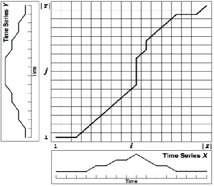
Dynamic Time Warping is an algorithm that is applied to temporal sequences to find the similarities between them. Unlike the Euclidean distance, Dynamic Time Warping is not susceptible to distortions in the time-axis. DTW finds the optimal match between the two time series. These series are „warped‟ non-linearly against the time-axis in order to determine the similarity between them which is independent of their variations with respect to time. DTW was originally developed for speech recognition applications. Dynamic Time Warping algorithm can be explained in the following way. Consider two time series X and Y of the same length n.

That is,

(2)

[image:2.595.59.265.74.177.2]

35 𝑌 = 𝑦1, 𝑦2, 𝑦3, … … … … . . , 𝑦𝑛

Fig. 1: Alignment of two time series where aligned points are indicated by arrows

By constructing a 𝑛 × 𝑛 cost matrix whose every 𝑖, 𝑗 𝑡𝑕 element is the distance between xi and yj, find a path through

this matrix such that it minimizes the cumulative distance. This path gives the optimal alignment between the two time series. To find the distance between xi and yj, test with various

distance measures like Euclidean distance, Manhattan Distance and so on. The effect of using these different distance measures will be evident in the classification step.

Fig. 2: Cost matrix to minimize the cumulative distance between two time series

Consider W to be the warping-path.

𝑊 = 𝑤1, 𝑤2, 𝑤3, … … … , 𝑤𝑘

Where, wkrepresents the distance between point i of X and

point j of Y.

The DTW between the time series X and Y can be calculated as:

𝐷𝑇𝑊 𝑋, 𝑌 = min⁡_{(𝑊 𝑥𝑖, 𝑦𝑗 )}

Although DTW is efficient in finding the similarity between the time series, its time complexity of O(n2) makes it rather computational intensive for large time series.

In order to reduce the time complexity of DTW algorithm, LB Keogh Lower Bound function of Dynamic Time Warping is used as it is linear in nature. The LB Keogh function is given as:

𝐿𝐵𝐾𝑒𝑜𝑔 𝑕 𝑋,𝑌 =

𝑥𝑖 − 𝑈𝑖 2 𝑖𝑓 𝑥𝑖 > 𝑈𝑖 𝑥𝑖 − 𝐿𝑖 2 𝑖𝑓 𝑥𝑖 < 𝐿𝑖

0 𝑜𝑡𝑕𝑒𝑟𝑤𝑖𝑠𝑒

𝑛

𝑖=1

Where, Ui and Li are the upper bound and lower bound of the

time series X.

This reduces the time complexity of the DTW algorithm to O(n).

The 𝐿𝐵𝐾𝑒𝑜𝑔 𝑕 𝑋,𝑌 ≤ 𝐷𝑇𝑊(𝑋, 𝑌), and hence eliminate the time

series that cannot be more similar than the current most similar time series. By this way, many unnecessary Dynamic Time Warping computations are reduced, thus reducing the time complexity of the DTW algorithm.

2.2 K-Nearest Neighbor

K-Nearest Neighbor (KNN) is an instance-based algorithm that stores all the available inputs and classifies the new input based on a similarity measure. It is also called as a „lazy learner‟ as there is no model building for classification. KNN is non-parametric and classification is carried out by majority voting of the neighbors of an input object. The training data for KNN are vectors in a multidimensional feature space, each having its associated class label. The 1-Nearest Neighbor is the most intuitive among all nearest neighbor type classifiers as it assigns a point to the class of its nearest neighbor in the feature space. As the training data size increases and approaches infinity, the 1NN guarantees an error rate of no worse than twice the Bayes error rate. This is the reason why 1NN is popularly used for classification purposes.

In this paper, 1-Nearest Neighbor has been implemented using Dynamic Time Warping as its distance measure.

Following are the steps of K-Nearest Neighbor for Time Series Classification:

1. Initialize the value of K=1

2. Compute the distance between the test time series and the training time series samples using Dynamic Time Warping as the distance measure

3. Sort the distances

4. Consider the 1-Nearest Neighbor

5. Assign the class of the nearest neighbor of the training time series to the test time series

This gives the classification of the test time series by assigning appropriate labels to them.

Let‟s see the effect of various distance measures used with Dynamic Time Warping algorithm that affect the overall classification accuracy of the system.

2.3 Distance Measures

2.3.1 Euclidean Distance

Euclidean distance is the most popularly used distance measure. It is the ordinary straight-line distance between two points. For time series, the distance is calculated as the square root of the sum of the squares of the differences between the corresponding training and test series of the same length. If in case the series are of different lengths, zero-padding is done for equivalent length. For the two series X and Y both of length n, Euclidean distance can be calculated as:

𝑑𝐸 = 𝑥𝑖 − 𝑦𝑖 2

𝑛

[image:2.595.59.274.308.495.2]

(3)

36

2.3.2 Normalized Euclidean Distance

The normalized Euclidean distance is calculated by dividing the Euclidean distance calculated between the series X and Y by the square root of the length of the series, i.e. n. It can be calculated as:

𝑑𝑁 =𝑑𝐸 𝑛

2.3.3 Manhattan Distance

Manhattan distance is also known as City-Block distance or Taxi-Cab distance. Unlike Euclidean distance, Manhattan distance cannot move with the points diagonally i.e. the length of the shortest path between two points, instead it moves vertically and horizontally by calculating the distances along each dimension. The Manhattan distance can be calculated as follows:

𝑑𝑀 = 𝑥𝑖 − 𝑦𝑖

𝑛

𝑖=1

2.3.4 Canberra Distance

Canberra distance is the weighted version of Manhattan distance. It has been used as a metric for comparing ranked lists. The Canberra distance between vectors X and Y in an n-dimensional real vector space can be calculated as:

𝑑𝐶 = _{𝑥𝑖 + |𝑦𝑖|} 𝑥𝑖 − 𝑦𝑖

𝑛

𝑖=1

3. TIME SERIES CLASSIFICATION

STEPS

1. Identify the input datasets for training and testing. 10 datasets from the UCR Time Series Archive [7] have been considered for this experiment.

2. Calculate the 1-Nearest Neighbor for classification by using the Dynamic Time Warping algorithm for calculating the similarity between the time series.

3. While calculating the Dynamic Time Warping distance, change the distance calculation step by considering different distance measures like Euclidean distance, Normalized Euclidean distance, Manhattan distance and Canberra distance.

4. Assign the label of the 1-Nearest Neighbor to the time series and return the classification accuracy for each distance measure.

Two important steps for Time Series Classification:

[1] Finding the similarity between the time series using Dynamic Time Warping

[2] Using the results obtained in step [1] for classification using the K-Nearest Neighbor algorithm.

For the Dynamic Time Warping algorithm, experiment has been performed by using different distance measures such as the Euclidean distance, Manhattan distance, Normalized Euclidean distance and Canberra Distance, to test its effect on the classification step. The results showed that using different distance measures for Dynamic Time Warping indeed affects the accuracy results of the classification algorithm. Not only the accuracy, even the time taken for the classification differs with every distance measure. This is mainly due to the fact that there are lesser candidates for comparison for the test data due to the properties of the different distance measures.

The experiment was carried out using Python 3.6 software package on Windows OS with 8GB RAM, 3.40 GHz Quadcore i7 processor.

4. PERFORMANCE MEASURES

Following are the performance measures considered to evaluate the classification performance of the proposed system.

4.1 Precision

Precision can be seen as a measure of exactness or quality. High precision means that an algorithm returned substantially more relevant results than irrelevant. Precision for time series classification can be calculated as:

𝑃𝑟𝑒𝑐𝑖𝑠𝑖𝑜𝑛 = 𝑇𝑟𝑢𝑒 𝑃𝑜𝑠𝑖𝑡𝑖𝑣𝑒

𝑇𝑟𝑢𝑒 𝑃𝑜𝑠𝑖𝑡𝑖𝑣𝑒 + 𝐹𝑎𝑙𝑠𝑒 𝑃𝑜𝑠𝑖𝑡𝑖𝑣𝑒 Where,

True Positive – Number of time series that have been correctly classified as belonging to Class „x‟

False Positive - Number of time series that have been incorrectly classified as belonging to Class „x‟

4.2 Recall

Recall is a measure of completeness or quantity. Recall can be calculated as follows:

𝑅𝑒𝑐𝑎𝑙𝑙 = 𝑇𝑟𝑢𝑒 𝑃𝑜𝑠𝑖𝑡𝑖𝑣𝑒

𝑇𝑟𝑢𝑒 𝑃𝑜𝑠𝑖𝑡𝑖𝑣𝑒 + 𝐹𝑎𝑙𝑠𝑒 𝑁𝑒𝑔𝑎𝑡𝑖𝑣𝑒

Where,

True Positive – Number of time series that have been correctly classified as belonging to Class „x‟

False Negative – Number of time series that belong to class „x‟ but have been classified as belonging to class „y‟

4.3 F1-score

F1 score is the weighted average of precision and recall. F1 is more useful than calculating the Accuracy measure in case of uneven class distribution. F1 score can be calculated as:

𝐹1 𝑠𝑐𝑜𝑟𝑒 = 2𝑝𝑟𝑒𝑐𝑖𝑠𝑖𝑜𝑛 × 𝑟𝑒𝑐𝑎𝑙𝑙 𝑝𝑟𝑒𝑐𝑖𝑠𝑖𝑜𝑛 + 𝑟𝑒𝑐𝑎𝑙𝑙

5. CLASSIFICATION RESULTS

5.1 Summary of Performance Metrics

(P-Precision, R-Recall, F1-F1 Score)

Table 1. Summary for Synthetic Control Dataset

Dataset Name

Distance Measures

Performance Measures

Time Taken

(s)

P R F1

Synthetic Control #Classes =

6 #Training

Series = 300 #Test Series =

300

Euclidean

Distance 0.99 0.99 0.99 279.42 Normalized

Euclidean 0.98 0.99 0.99 174.22 Manhattan

Distance 0.97 0.97 0.97 302.54

Canberra

(4)

[image:4.595.307.546.75.305.2]

37

Table 2. Summary for Gun-Point Dataset

Dataset Name Distance Measures Performance Measures Time Taken (s)

P R F1

Gun-Point #Classes =

2 #Training Series = 50

#Test Series =

150

Euclidean

Distance 0.98 0.98 0.98 156.32 Canberra

Distance 0.91 0.90 0.91 170.33

Table 3. Summary for CBF Dataset

P R F1

CBF #Classes =

#Test Series =

900

Euclidean

Distance 0.90 0.90 0.90 1011

Table 4. Summary for Trace Dataset

P R F1

Trace #Classes=4 #Training Series = 100 #Test Series = 100 Euclidean

[image:4.595.53.292.80.222.2]

Distance 0.92 0.92 0.92 114.45

Table 5. Summary for Fish Dataset

P R F1

Fish #Classes = 7 #Training Series = 175 #Test Series = 175 Euclidean

Distance 0.96 0.97 0.97 179.27

Canberra

Distance 0.91 0.91 0.91 182.39

Table 6. Summary for Car Dataset

P R F1

Car #Classes

= 4

Euclidean

Distance 0.98 0.99 0.99 57.43 Normalized 0.98 0.99 0.99 32.45

#Training Series = 60 #Test Series = 60 Euclidean Manhattan

Distance 0.97 0.97 0.97 64.29

Canberra

Distance 0.90 0.90 0.90 71.56

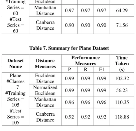
Table 7. Summary for Plane Dataset

P R F1

Plane #Classes = 7 #Training Series = 105 #Test Series = 105 Euclidean

Distance 0.96 0.96 0.96 110.35

Canberra

Distance 0.92 0.92 0.92 118.88

Table 8. Summary for Beef Dataset

P R F1

Beef #Classes = 5 #Training Series = 30 #Test Series = 30 Euclidean

Distance 0.98 0.98 0.98 31.43

Canberra

Distance 0.91 0.91 0.91 36.76

Table 9. Summary for Coffee Dataset

P R F1

Coffee #Classes =

#Test Series = 28

Euclidean

Distance 0.89 0.90 0.90 38.43

Table 10. Summary for Olive Oil Dataset

P R F1

Olive Oil #Classes =

#Test Series = 30

Euclidean

[image:4.595.50.286.381.760.2]

(5)

[image:5.595.60.537.62.699.2]

38

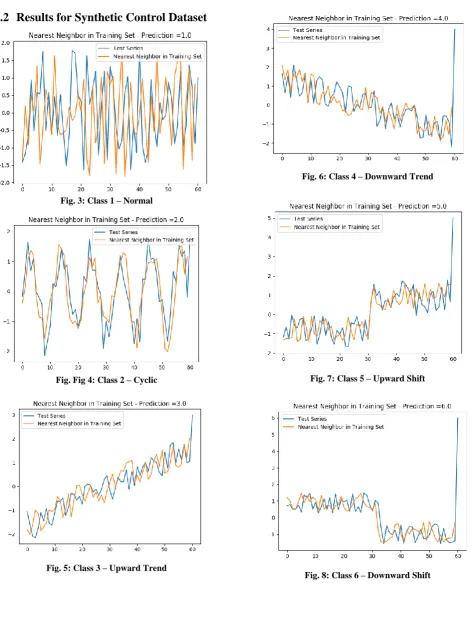
5.2 Results for Synthetic Control Dataset

Fig. 3: Class 1 – Normal

Fig. Fig 4: Class 2 – Cyclic

[image:5.595.322.527.78.247.2]

Fig. 5: Class 3 – Upward Trend

[image:5.595.56.269.89.472.2]

Fig. 6: Class 4 – Downward Trend

Fig. 7: Class 5 – Upward Shift

[image:5.595.325.524.270.456.2]

(6)

39

6. OBSERVATIONS

From the results given in the tables Table 1 - Table 10, the following observations can be noted.

1. Time series classification using Euclidean distance for DTW algorithm gives the best classification result among all the distance measures. Also, the time complexity is O(n), as it is with DTW.

2. The next distance measure that gives good classification accuracy is Normalized Euclidean Distance. Although its accuracy is slightly lesser than that of Euclidean distance, the time required is nearly half of that of Euclidean Distance. In situations of time-intensive time series classification problems, using Normalized Euclidean distance can significantly reduce the computation time. Even though the time complexity is O(n), in cases of extremely large amounts of data, such as Big data, Normalized Euclidean Distance might be preferable over Euclidean distance.

3. Manhattan distance gives acceptable classification results with DTW algorithm though it‟s not as efficient as the Euclidean distance or Normalized Euclidean Distance. The time required is similar to that of Euclidean distance. So in comparison to Manhattan distance, Euclidean distance is more preferred. The advantage of Manhattan distance over Euclidean distance is that it is comparatively easier to calculate.

4. Among all the distance measures, Canberra distance performs the worst. Though the classification results are average, but when compared with the other distance measures like Euclidean distance, Normalized Euclidean distance and Manhattan distance, Canberra distance surely doesn‟t provide optimal results.

7. CONCLUSION

Time series classification has attracted many researches in the recent decade. Using Dynamic Time warping similarity measure for time series classifications has been proved to produce good results for time series classification. Dynamic Time Warping algorithm inherently uses distance measures to calculate the similarity between the time series. Through this experiment, it is evident that different distance measures provide different classification results. Among them, Euclidean distance proved to give the best result followed by

Normalized Euclidean Distance and Manhattan Distance. Canberra Distance resulted in average classification accuracy. For time-intensive time series classification, Normalized Euclidean distance can be more beneficial than Euclidean distance. Further work can be done using other correlation based distance measures. Also, the approach for Nearest Neighbor can be centroid-based or medoid-based to further reduce the computations.

8. ACKNOWLEDGMENTS

I would like to convey my heartfelt gratitude to my guide Prof. K. C. Waghmare for encouraging me to carry out this research on Time Series Classification and for all the guidance provided to me during this research.

9. REFERENCES

[1] Bar-Joseph. Z., Gerber, G., Gifford, D., Jaakkola T & Simon. I. (2002). A new approach to analyzing gene expression time series data. In Proceedings of the 6th Annual International Conference on Research in Computational Molecular Biology. pp. 39-48.

[2] Itakura, F. (1975). Minimum prediction residual principle applied to speech recognition. IEEE Trans. Acoustics, Speech, and Signal Proc., Vol. ASSP-23, pp. 52-72.

[3] L. Wei and E. Keogh, “Semi-supervised Time Series Classification”, Proceedings of the 12th ACM SIGKDD International Conference on Knowledge Discovery and Data Mining, ACM 2006, pp. 748-753.

[4] Rohit J. Kate, “Using Dynamic Time Warping as Features for Improved Time Series Classification”, Data mining and Knowledge Discovery, March 2016, pp. 283-312.

[5] Ratanamahatana, Chotirat Ann, and Eamonn Keogh. "Making time-series classification more accurate using learned constraints." Proceedings of the 2004 SIAM International Conference on Data Mining. Society for Industrial and Applied Mathematics, 2004, pp. 11-22.

[6] Berndt, D. & Clifford, J. (1994). Using dynamic time warping to find patterns in time series. AAAI-94 Workshop on Knowledge Discovery in Databases. pp. 229-248.

[7] Yanping Chen, Eamonn Keogh, Bing Hu, Nurjahan Begum, Anthony Bagnall, Abdullah Mueen and Gustavo Batista, “The UCR Time Series Classification Archive”, 2015.