Lagrange’s Spectral Collocation Method for Numerical Approximations of Two Dimensional Space Fractional Diffusion Equation

ISSN Online: 2161-1211 ISSN Print: 2161-1203

DOI: 10.4236/ajcm.2018.82010 Jun. 13, 2018 121 American Journal of Computational Mathematics

Lagrange’s Spectral Collocation Method for

Numerical Approximations of

Two-Dimensional Space Fractional Diffusion

Equation

Hasib Uddin Molla

1*

_{, Mushfika Hossain Nova}

2

1_{Department of Mathematics, University of Dhaka, Dhaka, Bangladesh}

2_{Institute of Natural Sciences, United International University, Dhaka, Bangladesh}

Abstract

Due to the ability to model various complex phenomena where classical cal-culus failed, fractional calcal-culus is getting enormous attention recently. There are several approaches available for numerical approximations of various types of fractional differential equations. For fractional diffusion equations spectral collocation is one of the efficient and most popular approximation techniques. In this research, we introduce spectral collocation method based on Lagrange’s basis polynomials for numerical approximations of two-dimensional (2D) space fractional diffusion equations where spatial frac-tional derivative is described in Riemann-Liouville sense. We consider four different types of nodes to generate Lagrange’s basis polynomials and as col-location points in the proposed spectral colcol-location technique. Spectral collo-cation method converts the diffusion equation into a system of ordinary dif-ferential equations (ODE) for time variable and we use 4th _{order Runge-Kutta} method to solve the resulting system of ODE. Two examples are considered to verify the efficiency of different types of nodes in the proposed method. We compare approximated solution with exact solution and find that Lagrange’s spectral collocation method gives very high accuracy approximation. Among the four types of nodes, nodes from Jacobi polynomial give highest accuracy and nodes from Chebyshev polynomials of 1st _{kind give lowest accuracy in the} proposed method.

Keywords

Lagrange’s Spectral Method, 2D Fractional Diffusion Equation, Collocation Method

How to cite this paper: Molla, H.U. and Nova, M.H. (2018) Lagrange’s Spectral Collocation Method for Numerical Ap-proximations of Two-Dimensional Space Fractional Diffusion Equation. American Journal of Computational Mathematics, 8, 121-136.

https://doi.org/10.4236/ajcm.2018.82010 Received: February 9, 2018

Accepted: June 10, 2018 Published: June 13, 2018 Copyright © 2018 by authors and Scientific Research Publishing Inc. This work is licensed under the Creative Commons Attribution International License (CC BY 4.0).

http://creativecommons.org/licenses/by/4.0/

DOI:10.4236/ajcm.2018.82010 122 American Journal of Computational Mathematics

1. Introduction

Theory of Fractional calculus is almost of same age as that of the classical lus. The concept of a fractional derivative initiates the theory of fractional calcu-lus when this concept first appeared in a letter of L’Hospital to Leibnitz in 1695 [1]. But in 1819, Lacroix first mentioned the derivative of arbitrary order in a text [2]. Later from 1832 Liouville [3] starts to provide the initial foundations of the fractional calculus. A brief history and fundamental theory of fractional cal-culus can be found in [4]. Though many important physical processes in almost all branches of sciences can be described using various tools of classical calculus, there are also many complex phenomena that cannot be modeled using classical calculus. Being one of the most important generalizations of classical calculus, fractional calculus has been used to describe many such complex processes re-cently. In last few decades, scientists and engineers have found fractional order derivative very powerful to describe problems in anomalous diffusion, signal processing, control processing, fractional stochastic system and viscoelasticity. In space fractional diffusion equation, spatial derivative of order

1

< <

α

2

rep-laces the classical second order spatial derivative in classical diffusion equation and results into super diffusive flow model. Unlike classical order derivative, fractional derivative has several kinds of definitions such as Caputo, Rie-mann-Liouville, Grünwald-Letnikov and Riesz. Detailed discussion about vari-ous definitions of fractional derivative can be found in [5][6].

DOI: 10.4236/ajcm.2018.82010 123 American Journal of Computational Mathematics Loghmani applied collocation technique with Gauss-Lobatto nodes whereas Xie et al. used tau method to determine expansion coefficients. For numerical ap-proximations of 1D fractional diffusion equation Bahsi and Yalcinbas [10] cho-sen Fibonacci polynomials to express the trial solution in both space and time domain and then used evenly spaced collocation points. Pirim and Ayaz [11] al-so chosen evenly spaced collocation points but expressed the trial al-solution in terms of Hermite polynomials for approximations of fractional order system of differential equations. Huang and Zheng [12] used Jacobi polynomials and La-grange’s basis polynomials for spectral approximations of 1D space fractional diffusion equations and used Gauss-Lobatto nodes for collocation. Doha et al. [13] presented spectral tau method for 1D space fractional diffusion equation where they expand the solution by Jacobi polynomials. For spectral expansion of trial solution for time fractional diffusion equations Lagrange interpolation po-lynomials are used in both 1D space and time domain by Huang [14]. For collo-cation purpose he chose Jacobi-Gauss nodes for time domain and for space do-main he chosen Gauss-Lobatto nodes. Zayernouri and Karniadakis [15] intro-duced fractional Lagrange interpolants and developed a new fractional spectral collocation method for 1D fractional differential equations. Krishnaveni et al. [16] proposed a hybrid method for 1D space fractional diffusion equation where trial solution is approximated by spectral expansion of fractional shifted Legen-dre polynomials. To approximate the solution of 2D space fractional diffusion equation by spectral collocation method Bhrawy [17] used shifted Legendre po-lynomials and Gauss-Lobatto nodes for 2D space domain. Other numerical me-thods such as ADI and Finite-Difference meme-thods [18] [19] [20] [21] [22] are also very efficient for 2D problems.

DOI:10.4236/ajcm.2018.82010 124 American Journal of Computational Mathematics The performances in terms of resultant accuracy by four sets of nodes in pro-posed Lagrange’s spectral collocation method are illustrated and compared through numerical examples. Similar investigation on 1D space fractional diffu-sion equation is carried out by Nova et al. [24] recently.

Remaining parts of this paper are organized as follows: Section 2 contains the preliminaries of different polynomials and fractional derivative. Then in Section 3, detailed formulations of Lagrange’s spectral method for 2D space fractional diffusion equation are given. Next in Section 4, numerical examples are consi-dered to demonstrate the accuracy of the proposed method and to compare the performance of four types of nodes. Finally, conclusion is drawn about this re-search in Section 5.

2. Preliminaries

In this section, we present a brief introduction of Legendre, Jacobi and Cheby-shev polynomials of 1st _{and 2}nd _{kinds. Also short description of Lagrange’s basis} polynomials and Caputo’s fractional order derivative are given.

Legendre Polynomials: The nth degree Legendre polynomial P wn

( )

over

the domain

[

−1,1

]

are explicitly defined as

( )

0 1 1 2 k n n k

n n w

P w k k = − −    −  = _{   }     

∑

(1)

Chebyshev Polynomials of 1st _{Kind: The nth degree Chebyshev polynomials} of 1st _kind

( )

n

T w over the domain

[

−1,1

]

_{are explicitly defined as}

( )

2

(

2

)

0 1 2 n k n n k n

T w w w

k       − =   = _{ } −  

∑

(2)

Chebyshev Polynomials of 2nd _{Kind: The nth degree Chebyshev polynomials} of 2nd _kind

( )

n

U w over the domain

[

−1,1

]

_{are explicitly defined as}

( )

2

(

2

)

0 1 1 2 1 n k n n k n

U w w w

k       − = +   = _{ } − +  

∑

(3)

Jacobi Polynomials: The nth degree Jacobi polynomials i j,

( )

n

P w on the in-terval

[

−1,1

]

are defined as

( )

₍

(

)

₎

(

₍

₎

)

,

0

1 1 1

! 1 1 2

k r i j n k r

i n i j r k w

P w

k

i i j n = i k

Γ + +  Γ + + + +  − 

= _{   }

Γ + + +

∑

  Γ + +   (4)

Lagrange Basis Polynomials: For

(

p+1

)

_points x x₁, , , ,₂  x xp p+₁ La-grange basis polynomials L x nn

( )

; =1,2, , p+1 each of degree p are defined

as follows:

( )

1

(

)

1

p k k

h x + x x

=

=

∏

−

( )

_{( )(}

( )

₎

; 1,2, , 1

n

n

h x

L x n p

h x x x

= = +

DOI: 10.4236/ajcm.2018.82010 125 American Journal of Computational Mathematics with the property L xn

( )

m =

δ

mn, where δmn is the Kronecker delta function.

Here h x′

( )

_{is the derivative of} h x

( )

.

Riemann-Liouville Fractional Derivative: Riemann-Liouville fractional de-rivative operator of order α is denoted by Dα _{and defined by:}

( )

₍

₎

(

)

1

( )

0

1 d _{d , 0}

Γ d

x m

m m

D f x x t f t t

m x

α

α _α

α

− −

= − >

−

∫

(6)

with m− < <1

α

m m, ∈_.

Then for

α

>0,m− < <1

α

m m, ∈_{ and} p≥0

(

)

(

Γ 1

)

Γ 1

p p p

D x x

p

α α

α

−

+ =

− + (7)

where =

{

1,2,3,

}

.

Like classical integer order derivative, Riemann-Liouville fractional order de-rivative is also a linear operator.

3. Lagrange’s Spectral Collocation Method

Lagrange’s Spectral Collocation method for numerical approximations of 2D space fractional diffusion equation will be presented in this section. In this re-search, we consider following form of diffusion equation

(

)

₍

₎

(

)

₍

₎

(

)

(

)

1 2

, , , , , ,

, ,

, , ; 0 , 0 , 0

u x y t u x y t u x y t

g x y g x y

t x y

f x y t x a y b t

α β

α β

∂ ∂ ∂

= +

∂ ∂ ∂

+ ≤ ≤ ≤ ≤ >

(8)

subject to the initial condition

(

, ,0

)

3

( )

, ; 0 , 0

u x y =g x y ≤ ≤x a ≤ ≤y b ₍₉₎ and non-homogeneous Dirichlet’s boundary conditions

(

0, ,

)

4

( ) (

, , , ,

)

5

( )

, ; 0 , 0

u y t =g y t u a y t =g y t ≤ ≤y b t≥ ₍₁₀₎

(

,0,

)

6

( ) (

, , , ,

)

7

( )

, ; 0 , 0

u x t =g x t u x b t =g x t ≤ ≤x a t≥ ₍₁₁₎

Here g x y1

( )

, and g x y2

( )

, are the diffusion coefficients, f x y t

(

, ,

)

is the force function and u x y t

(

, ,

)

is the unknown function to be solved.

For numerical approximations of Equation (8) by Lagrange’s spectral colloca-tion method we first divide the interval

[ ]

0,a of space domain x into p subin-tervals and interval

[ ]

0,b of y domain into q subinterval by means of following nodes:

1 2 3 1

0=x x x, , , , , x xp p+ =a (12)

1 2 3 1

0=y y y, , , , , y yp p+ =b (13) These nodes can be chosen with no specific pattern and from anywhere in the domain. Then using these nodes

{ }

1

1

i p i i

x = +

= from x-domain we form Lagrange’s basis polynomials L x nn

( )

; =1,2, , , p p

(

+1

)

each of degree p and using nodes

{ }

1

1

j q j j

DOI:10.4236/ajcm.2018.82010 126 American Journal of Computational Mathematics

( )

; 1,2, , ,

(

1

)

m

L y m′ =  q q+ each of degree q. Now at these nods Lagrange’s ba-sis polynomials satisfies L xn

( )

i =

δ

ni and L ym′

( )

j =

δ

mj. These nodes are also

used as collocation points in the later part of this section.

Now as spectral approximation of u x y t

(

, ,

)

, the solution of Equation (8) we consider trial solution u x y t

(

, ,

)

in the form

(

)

1 1

( ) ( ) ( )

1 1

, , p q n m

n m n m

u x y t + + v t L x L y

= =

′

=

∑∑

 (14)

( ) ( )

( )

( )

( )

( ) ( ) ( )

( ) ( )

( )

( )

( )

1

1 1

1 1

1 2 2

1 1 1 1

2

m m

q p q

p n

m m p m n

m n m

p

n n

q q n

n

v t L x v t L x L y v t L x L y

v t L y v t L y L x

+ + + = = = + + =   ′ ′ = _ + _ +  ′ ′  + _ + _

∑

∑ ∑

∑

(15)

Here Lagrange’s basis polynomials L xn

( )

and L ym′

( )

are used as the basis

functions in spectral approximations and

{

n

( )

}

n1,2, , , 1_{1,2, , , 1}p p mv t _{m q q}

= +

= +



 are the expansion

coefficients needed to be determined. Now we write the residual R x y t

(

, ,

)

for Equation (8) as

(

)

(

)

( )

(

)

( )

(

)

(

)

1 2 , , , , , , , , , , , ,

u x y t u x y t R x y t g x y

t x

u x y t

g x y f x y t y α α β β ∂ ∂ = − ∂ ∂ ∂ − − ∂  

 (16)

where

( ) ( )

( )

( )

( )

( ) ( ) ( )

( ) ( )

( )

( )

( )

1 1 1 1 1 1 1 2 2

1 1 1

2

q

p

m m p

m p q n m n m p n n q q n m n m n

u _{v t L x v t L x L y} x

v t L x L y

v t L y v t L y L x

α α α α α α + + + = = = + + = ∂ _{  ′} = _ + _ ∂ ′ +  ′ ′  + _ + _

∑

∑ ∑

∑

 (17)

( ) ( )

( )

( )

( )

( ) ( ) ( )

( ) ( )

( )

( )

( )

1 1 1 1 1 1 2 2

1 1 1 1

2

q

p

m m p m

m

p q

n

m n m

n m

p

n n

q q n

n

u _{v t L x v t L x L y} y

v t L x L y

v t L y v t L y L x β β β β β β + + + = = = + + = ∂ _{  ′} = _ + _ ∂ ′ +  ′ ′  + _ + _

∑

∑ ∑

∑

 (18)

( ) ( )

( )

1 1 1 1 d d n p q m n m n m v t

u _{L x L y}

t t

+ +

= =

∂ _{= ′}

∂

∑∑

 ₍₁₉₎

Here L xαn

( )

is the α order Riemann-Liouville fractional derivative of

( )

n

L x with respect to x and L ym′β

( )

is the β order Riemann-Liouville

frac-tional derivative of L xm′

( )

with respect to y.

To determine the expansion coefficients we chose collocation technique and for this we force the residual equation at Equation (16) to be zero at

(

p− ×1

) (

q−1

)

_{interior points}

{

(

)

}

2,3, , 1,

2,3, , 1,

, i p p

i j _{j q q}

x y =₌  −₋

DOI: 10.4236/ajcm.2018.82010 127 American Journal of Computational Mathematics force the trial solution to satisfy the boundary conditions Equation (10) & (11) at the boundary lines.

First by setting the residual at Equation (16) to be zero at the interior points of the spatial domain, we have the equation

(

)

(

)

(

) (

)

(

) (

) (

)

1 2 , , , , , , , , ,

, , , 0

i j i j

i j i j

i j

i j i j

x y t x y t

R x y t g x y

t x

u u

u x y t

g x y f x y t

y α α β β ∂ ∂ = − ∂ ∂ ∂ − − = ∂  

 (20)

for i=2,3, ,_ p−1,p _and j=2,3, ,_ q−1,q _with

(

)

1

₍

₎

_{( )}

_{( )}

_{( )}

_{( )}

1

1 2 2

, ,

, ,

q p q

i j n

i j m n i j

m m n m m

u x y t

k m x t L y v t L x L y x α α α + = = = ∂ ′ ′ = + ∂

∑

∑ ∑

 (21)

(

)

_{( ) ( )}

_{( )}

₍

₎

_{( )}

2

2 2 2

, ,

, ,

p q p

i j n

m n i m j j n i

n m n

u x y t

v t L x L y k n y t L x y β β β = = = ∂ ′ = + ∂

∑ ∑

∑

 (22)

(

)

_{( )}

_{( )}

( )

2 2

, , d

d

m

n

p q

i j m

n i j

n m

u x y t v t

L x L y

t = = t

∂ ′ = ∂

∑ ∑

 (23) where

(

)

1

( ) ( )

1

( )

( )

1 , ,i m 1 i pm p1 i

k m x t v t L xα +v t Lα x +

 

=_ + _{ (24)}

(

)

( )

( )

( )

( )

2 , ,j 1n 1 j q1n q1 j

k n y t v t L yβ v t Lβ y

+ +

 ′ ′ 

=_ + _ (25)

Thus Equation (20) gives us the following system of ODE for time variable t

( )

_{( )}

₍

₎

_{( ) ( )}

₍

₎

_{( )}

_{( )}

, 1 2

2 2

d

, ,

d

i _{p q}

j n i

i j i j j n i i j m m j

n m

v t

a t g x y v t L x g x y v t L y t

α β

= =

′

= +

∑

+

∑

₍₂₆₎

with

( )

(

)

(

)

(

) (

) (

)

, 1 , 1 , , 2 , 2 , , , ,

i j i j i i j j i j

a t =g x y k j x t⋅ +g x y k i y t⋅ + f x y t ₍₂₇₎ Now forcing the trial solution to satisfy the initial condition Equation (9) at the interior points gives us the initial condition for system of ODE in Equation (26) as

( ) ( )

( )

3

(

)

2 2

0 ,

p q n

m n i j i j

n= m= v L x L ym g x y

′ =

∑ ∑

(28)

( )

0 3

(

,

)

i

jv g x yi j

⇒ = ₍₂₉₎

Now forcing the trial solution to agree with the boundary conditions for boundary lines x x= 1 and x x= p+1, that is, to satisfy the boundary conditions at Equation (10) gives

( ) ( )

( )

1 1 4 1 , q m m

m v t L y g y t +

=

′ =

∑

(30)

( ) ( )

( )

1 1 5 1 , q p m m

m v t L y g y t +

+

=

′ =

∑

(31)

DOI:10.4236/ajcm.2018.82010 128 American Journal of Computational Mathematics

( )

(

)

1

4 ,

mv t =g y tm and p+m1v t

( )

=g y t5

(

m,

)

for m=1,2, , , q q+1 (32)

Again forcing the trial solution to agree with the boundary conditions, now for boundary lines y y= 1 and y y= q+1, that is, to satisfy the boundary condi-tions at Equation (11) gives

( ) ( )

( )

1 6

2

,

p n

n

n= v t L x g x t =

∑

(33)

( ) ( )

( )

1 7

2 ,

p n

q n

n= +v t L x g x t =

∑

(34)

Now at the points x ii; =2,3, , p Equation (33) and (34) becomes

( )

(

)

1 6 ,

n

n

v t =g x t _{and 1}n

( )

₇

(

,

)

q+v t =g x tn for n=2,3, ,

(

p−1 ,

)

p (35)

System of ODE in Equation (26) with its initial condition Equation (29) can be solved for the value of expansion coefficients

{

n

( )

}

n2,3, ,_{2,3, ,}p

mv t _{m q} =

=



 at anyt T= F.

Rest of the values of expansion coefficients can be obtained from Equation (32) and (35). Replacing the values of expansion coefficients

{

n

( )

}

n1,2,3, , , 1_{2,3, , , 1}p p

mv t _{m q q}

= +

= +



 for

any particular t T= F into trial solution in Equation (14) will gives us the

ap-proximate solution u x y T

(

, , F

)

of Equation (8) in terms of Lagrange’s basis

po-lynomials L xn

( )

and L ym′

( )

.

4. Numerical Results

In this section, we consider two examples to apply the proposed method with four different types of nodes to investigate the accuracy of the method and nodes. System of ordinary differential equations in Equation (26) with initial condition Equation (29) is solved for the value of expansion coefficients

{

n

( )

}

n2,3, ,_{2,3, ,}p

mv t _{m q} =

=

  at

1

F

T = _{by 4}th _{order Runge-Kutta method with time step size 0.01.}

In both examples spatial domain was

[ ] [ ]

0,1× 0,1 _{and we consider} p q= =5. Four different types of nodes are thus derived as follows:

Since all the roots of Legendre, Jacobi and both kinds of Chebyshev polyno-mials are in the interval

(

−1,1

)

, to generate nodes

[ ]

1

1

k p k k

x = +

= over any arbitrary interval

[ ]

c d, , first we choose x c1= and xp+1=d . Then, the remaining

(

p−1

)

nodes are generated by shifting the roots of one of the above

(

p−1 th

)

degree polynomials into the interval

[ ]

c d, .

Since in both examples 2D space domain is square shaped and we consider

5

p q= = , following four sets of nodes are thus used for both x and y domain.

{

}

st

chebyshev 1 kind= 0,0.0380602,0.308658,0.691342,0.96194,1

{

}

nd

chebyshev 2 kind= 0,0.0954915,0.345492,0.654508,0.904508,1

{

}

legendre= 0,0.0694318,0.330009,0.669991,0.930568,1

{

}

jacobi= 0,0.1174723,0.357384,0.642616,0.882528,1

DOI: 10.4236/ajcm.2018.82010 129 American Journal of Computational Mathematics

(

, ,

)

(

, ,

) (

, ,

)

Er x y t = u x y t u x y t− We also consider maximum absolute error given by

( )

max

{

(

, , : 0

)

,0

}

AE

M t = Er x y t ≤ ≤x a ≤ ≤y b

For numerical simulation we develop codes for the proposed method using MATLAB.

Example 1: Consider the diffusion equation [17] [18]

(

)

₍

₎

(

)

₍

₎

(

)

(

)

1.8 1.6

1 1.8 2 1.6

, , , , , ,

, ,

, , ; 0 1, 0 1, 0

u x y t u x y t u x y t

g x y g x y

t x y

f x y t x y t

∂ ∂ ∂

= +

∂ ∂ ∂

+ ≤ ≤ ≤ ≤ >

with boundary conditions

(

_{0, ,}

)

_{0, 1, ,}

(

)

_e t 3.6_{; 0 1, 0}

u y t ₌ u y t ₌ −y _{≤ ≤}y t_≥

(

_,0,

)

_0,

(

_,1,

)

_et 3_{; 0 1, 0}

u x t ₌ u x t ₌ −x _{≤ ≤}x t_≥ and with initial condition

(

_{, ,0}

)

3 3.6_{; 0 1, 0 1}

u x y =x y ≤ ≤x ≤ ≤y where

( )

( )

2.8

( )

_{( )}

2.6

(

)

(

)

3 3.6

1 2

2.2 2

, , , , , 1 2 e

6 Γ 4.6 ,

t

g x y ₌Γ x y g x y ₌ xy f x y t _{= − +} xy −x y The exact solution of this problem is given by _{u x y t}

(

_{, ,}

)

_=e−t_{x y}3 3.6_.

Applying the proposed Lagrange’s spectral collocation technique for

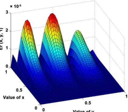
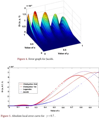
5

p q= = into Example 1 with four different types of nodes resulting surface graph of absolute local error Er x y

(

, ,1

)

are given into Figures 1-4. Then Fig-ure 5 contains the absolute local error curve Er x

(

,0.7,1

)

and Figure 6 con-tains the absolute local error curve Er

(

0.8, ,1y

)

for example 1.

Example 2: Consider the diffusion equation [17]

(

)

₍

₎

(

)

₍

₎

(

)

(

)

1.5 1.5

1 1.5 2 1.5

, , , , , ,

, ,

, , ; 0 1, 0 1, 0

u x y t u x y t u x y t

g x y g x y

t x y

f x y t x y t

∂ ∂ ∂

= +

∂ ∂ ∂

+ ≤ ≤ ≤ ≤ >

with boundary conditions

(

_{0, ,}

)

_{0, 1, ,}

(

)

_e t 3_{; 0 1, 0}

u y t ₌ u y t ₌ − y _{≤ ≤}y t_≥

(

_,0,

)

_0,

(

_,1,

)

_et 2_{; 0 1, 0}

u x t ₌ u x t ₌ −x _{≤ ≤}x t_≥ and with initial condition

(

_{, ,0}

)

2 3_{; 0 1, 0 1}

u x y =x y ≤ ≤x ≤ ≤y where

( )

( ) (

)

( )

( ) ( )

1 2

1.5 2.5

, 3 2 , , 4 ,

2 6

g x y =Γ − x g x y =Γ −y

(

_{, ,}

)

_et 2 32 ₄ 32

(

_{2 3}

)

3 f x y t ₌ − x _₋y _{+ −}y _y ₊ x x₋ y



 

 

 

[image:10.595.268.480.74.254.2] [image:10.595.269.480.291.481.2]

DOI:10.4236/ajcm.2018.82010 130 American Journal of Computational Mathematics Figure 1. Error graph for Chebyshev 1st _kind.

Figure 2. Error graph for Chebyshev 2nd _kind.

[image:10.595.269.480.518.702.2]

[image:11.595.204.535.71.463.2] [image:11.595.266.480.74.253.2]

DOI: 10.4236/ajcm.2018.82010 131 American Journal of Computational Mathematics Figure 4. Error graph for Jacobi.

Figure 5. Absolute local error curve for y=0.7_.

Figure 6. Absolute local error curve for x=0.8.

The exact solution of this problem is given by _{u x y t}

(

_{, ,}

)

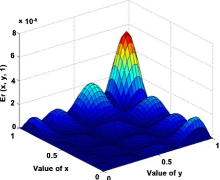
_=e−t_{x y}2 3 .

[image:11.595.211.538.481.629.2]

[image:12.595.259.488.71.256.2] [image:12.595.259.490.287.481.2]

DOI:10.4236/ajcm.2018.82010 132 American Journal of Computational Mathematics Figure 7. Error graph for Chebyshev 1st _kind.

Figure 8. Error graph for Chebyshev 2nd _kind.

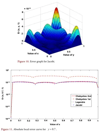
[image:12.595.260.486.518.703.2]

[image:13.595.203.536.66.505.2]

DOI: 10.4236/ajcm.2018.82010 133 American Journal of Computational Mathematics Figure 10. Error graph for Jacobi.

Figure 11. Absolute local error curve for y=0.7_.

local error curve Er x

(

,0.7,1

)

and Figure 12 contains the absolute local error curve Er

(

0.8, ,1y

)

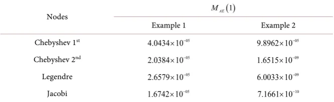
for Example 2.

Table 1 contains maximum absolute error MAE

( )

1 by four different sets of

nodes for both examples.

[image:13.595.264.485.71.258.2]

[image:14.595.208.537.62.252.2]

DOI:10.4236/ajcm.2018.82010 134 American Journal of Computational Mathematics Figure 12. Absolute local error curve for x=0.8.

Table 1. Maximum absolute error.

Nodes MAE( )1

Example 1 Example 2 Chebyshev 1st _{4.0434 10×} −05 _{9.8962 10×} −05 Chebyshev 2nd _{2.0384 10×} −05 _{1.6515 10×} −09 Legendre _{2.6579 10×} −05 _{6.0033 10×} −09 Jacobi _{1.6742 10×} −05 _{7.1661 10×} −10

x-domain performance of Jacobi nodes, Chebyshev 2nd_{, Legendre and Chebyshev} 1st _{nodes are found in decreased order.}

5. Conclusion

Spectral collocation method with Lagrange’s basis polynomials for approxima-tions of 2D space fractional diffusion equaapproxima-tions is introduced in this research. We used four different types of nodes generated from roots of Legendre, Jacobi, 1st _{and 2}nd _{kinds of Chebyshev polynomials. Nodes are used to form Lagrange’s} basis polynomials for spectral approximations and then as collocation points to determine the expansion coefficients. Performances of these four types of nodes in Lagrange’s spectral collocation method are investigated through two examples of 2D space fractional diffusion equation. Four types of nodes in proposed me-thod give very high accuracy approximations. We found that among four types of nodes Chebyshev 1st _{kind gives lowest accuracy and Jacobi nodes give highest} accuracy. We compared approximate solutions with exact solution and consi-dered absolute local error and maximum absolute error. Four different types of nodes showed consistent performance in both examples.

References

[image:14.595.207.540.305.407.2]

DOI: 10.4236/ajcm.2018.82010 135 American Journal of Computational Mathematics Georg Olm, 2, 301-302.

[2] Lacroix, S.F. (1819) Traité du Calcul Différentiel et du Calcul Intégral. 2nd Edition, Mme, Paris, Ve _{Courcier, Tome Troisiéme, 409-410.}

[3] Liouville, J. (1832) Mémoire sur quelques Quéstions de Géometrie et de Mécanique, et sur un nouveau genre de Calcul pour résoudre ces Quéstions. Journal de l'École Polytechnique, tome XIII, XXIe _{cahier, 1-69.}

[4] Ross, B. (1975) A Brief History and Exposition of the Fundamental Theory of frac-tional Calculus. In: Ross, B., Ed., Fracfrac-tional Calculus and Its Applications, Lecture Notes in Mathematics, Springer, Berlin, Heidelberg, 57, 1-36.

https://doi.org/10.1007/BFb0067096

[5] Herzallah, M.A.E. (2014) Notes on Some Fractional Calculus Operators and Their Properties. Journal of Fractional Calculus and Applications, 5, 1-10.

[6] Li, C., Qian, D. and Chen, Y.Q. (2011) On Riemann-Liouville and Caputo Deriva-tives. Discrete Dynamics in Nature and Society, 2011, Article ID: 562494.

https://doi.org/10.1155/2011/562494

[7] Khader, M.M. (2011) On the Numerical Solutions for the Fractional Diffusion Equ-ation. Communications in Nonlinear Science and Numerical Simulation, 16, 2535-2542.https://doi.org/10.1016/j.cnsns.2010.09.007

[8] Azizi, H. and Loghmani, G.B. (2013) Numerical Approximation for Space Fraction-al Diffusion Equation Chebyshev Finite Difference Method. Journal of Fractional Calculus and Applications, 4, 303-311.

[9] Xie, J., Huang, Q. and Yang, X. (2016) Numerical Solution of the One-Dimensional Fractional Convection Diffusion Equations Based on Chebyshev Operational Ma-trix. SpringerPlus, 5, 1149. https://doi.org/10.1186/s40064-016-2832-y

[10] Bahsi, A.K. and Yalcinbas, S. (2016) Numerical Solution and Error Estimations for the Space Fractional Diffusion Equation with Variable Coefficients via Fibonacci Collocation Method. SpringerPlus, 5, 1375.

https://doi.org/10.1186/s40064-016-2853-6

[11] Pirim, N.A. and Ayaz, F. (2016) A New Technique for Solving Fractional Order Systems: Hermite Collocation Method. Applied Mathematics, 7, 2307-2323.

https://doi.org/10.4236/am.2016.718182

[12] Huang, Y. and Zheng, M. (2013) Pseudo-Spectral Method for Space Fractional Dif-fusion Equation. Applied Mathematics, 4, 1495-1502.

https://doi.org/10.4236/am.2013.411202

[13] Doha, E.H., et al. (2014) The Operational Matrix Formulation of the Jacobi Tau Approximation for Space Fractional Diffusion Equation. Advances in Difference Equations, 2014, 231.https://doi.org/10.1186/1687-1847-2014-231

[14] Huang, F. (2012) A Time-Space Collocation Spectral Approximation for a Class of Time Fractional Differential Equations. International Journal of Differential Equa-tions, 2012, Article ID: 495202. https://doi.org/10.1155/2012/495202

[15] Zayernouri, M. and Karniadakis, G.E. (2014) Fractional Spectral Collocation Me-thod.SIAM Journal on Scientific Computing, 36, A40-A62.

https://doi.org/10.1137/130933216

[16] Krishnaveni, K., et al. (2016) An Efficient Fractional Polynomial Method for Space Fractional Diffusion Equations. Ain Shams Engineering Journal.

DOI:10.4236/ajcm.2018.82010 136 American Journal of Computational Mathematics [18] Tadjeran, C. and Meerschaert, M.M. (2007) A Second-Order Accurate Numerical

Method for the Two-Dimensional Fractional Diffusion Equation. Journal of Com-putational Physics, 220, 813-823.https://doi.org/10.1016/j.jcp.2006.05.030

[19] Liu, F., et al. (2013) Numerical Simulation for Two-Dimensional Riesz Space Frac-tional Diffusion Equations with Nonlinear Reaction Term. Central European Jour-nal of Physics, 11, 1221-1232.https://doi.org/10.2478/s11534-013-0296-z

[20] Nasrollahzadeh, F. and Hosseini, S.M. (2016) An Implicit Difference ADI Method for Two-Dimensional Space-Time Fractional Diffusion Equation. Iranian Journal of Mathematical Sciences and Informatics, 11, 71-86.

[21] Sweilam, N.H., Nagy, A.M. and Almajbri, T.F. (2014) Error Analysis of an Explicit Finite Difference Approximation for the Two-Dimensional Space Fractional Diffu-sion Equation. Journal of Fractional Calculus and Applications, 5, 1-10.

[22] Sweilam, N.H. and Almajbri, T.F. (2015) Large Stability Regions Method for the Two-Dimensional Fractional Diffusion Equation. Progress in Fractional Differen-tiation and Applications, 1, 123-131.

[23] Burden, R.L., Faires, D.J. and Burden, A.M. (2015) Numerical Analysis. Cengage Learning, Boston.

[24] Nova, M.H., Molla, H.U. and Banu, S. (2017) Comparison of Numerical Approxi-mations of One-Dimensional Space Fractional Diffusion Equation Using Different Types of Collocation Points in Spectral Method Based on Lagrange’s Basis Polyno-mials. American Journal of Computational Mathematics, 7, 469-480.