Abalone Age Prediction Problem: A Review

Abalone Age Prediction Problem: A Review

Kunj Mehta

Department of Computer Engineering KJ Somaiya College of Engineering

Vidyavihar, Mumbai, India

ABSTRACT

Abalones are sea snails or molluscs otherwise commonly called as ear shells or sea ears. Because of the economic importance of the age of the abalone and the cumbersome process that is involved in calculating it, much research has been done to solve the problem of abalone age prediction using its physical measurements available in the UCI dataset. This paper reviews the various methods like decision trees, clustering, SVM using Tomek links, CGANs and CasCor used in an attempt to solve it. Furthermore, in contrast to previous research that saw this as a classification problem, this paper approaches it as a linear regression problem and analyses the results.

General Terms

Machine Learning, Linear Regression, Neural Networks, Data Analysis.

Keywords

Abalone, Regression, SMOTE, RANSAC, CasCor, CasPer, UCI

1.

INTRODUCTION

Abalones are endangered marine snails that are found in the cold coastal waters worldwide, majorly being distributed off the coasts of New Zealand, South Africa, Australia, Western North America, and Japan [1]. They are considered a delicacy and a highly nutritious food and extensively consumed in certain parts of Latin America, France, New Zealand, Southeast Asia, China, Vietnam, Japan, and Korea. They are also commercially farmed as a source of mother-of-pearl. The shells of abalone are used for decorative purposes owing to their iridescence. This makes abalone a highly sought after commodity and economically significant.

The price of an abalone is positively correlated to its age.[2] However, determining the age of an abalone is a highly involved process. Rings are formed in the inner shell of the abalone as it grows, usually at the rate of one ring per year. Getting access to the rings of an abalone involves cutting the shell. After polishing and staining, a lab technician examines a shell sample under a microscope and counts the rings.

Because some rings are hard to make out using this method, 1.5 is traditionally added to the ring count as a reasonable approximation of the age of the abalone. Knowing the correct price of the abalone is important to both the farmers and consumers while knowing the correct age is important to environmentalists who seek to protect this endangered species. Due to the inherent inaccuracy in the manual method of counting the rings and thus calculating the age, researchers have tried to employ physical characteristics of the abalone such as sex, weight, height and length to determine its age. The corresponding dataset is found at UCI’s repository. [3]

Most of the research on the dataset has seen the abalone age prediction problem being categorized as a classification problem, that is, assigning a label to each example in the dataset. The label in this case is the number of rings of the abalone, which is a real number. This leads the classifier to distinguish among many classes and is thus bound to do poorly as can be seen in Zhengjie Wang’s results [4]. To improve upon this approach, the number of classes is reduced. However, doing so beats the purpose of easing the process of calculating age (and thereafter price), especially in the absence of concrete data about the degree of correlation between age and price. For instance, two ages belonging to one of the reduced class but nonetheless causing a large variation in price would render the reduced class model useless. To overcome the problems associated with the classification model, this paper experiments with regression models and analyses the performance. Mean Absolute Error (MAE) is used as the evaluation metric to downplay the significance of outliers (too young or too old abalones, which are rare in nature) and because it allows us to make a straightforward conclusion: a MAE below 0.5 would guarantee that the regressor has made a correct and useful prediction

2.

DATASET ANALYSIS

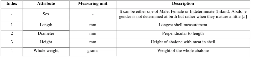
The abalone dataset is a dataset that contains measurements of physical characteristics of different abalones. It has 4177 instances. The physical characteristics along with the unit of its measurement in brackets are (Table 1) [3]:

Table 1. Description of variables in the abalone dataset

Index Attribute Measuring unit Description

- Sex - It can be either one of Male, Female or Indeterminate (Infant). Abalone gender is not determined at birth but rather when they mature a little [5]

1 Length mm Longest shell measurement

2 Diameter mm Perpendicular to length

3 Height mm Height of abalone with meat in shell

Index Attribute Measuring unit Description

5 Shucked weight grams Weight of just the meat

6 Viscera weight grams Gut weight (after bleeding)

7 Shell weight grams Weight of shell after being dried

8 Rings - This is the dependent variable (label). Number of rings + 1.5 gives age

Figure 1 shows the distribution of rings in the abalone dataset. It can be seen that the dataset is skewed with majority examples having rings in the range of 7-14 with very few examples having rings above 20. The exact number of examples in ascending order of number of rings in the examples is: (1, 1, 15, 57, 115, 259, 391, 568, 689, 634, 487, 267, 203, 126, 103, 67, 58, 42, 32, 26, 14, 6, 9, 2, 1, 1, 2, 0, 1).

Figure 1: Distribution of Rings Variable

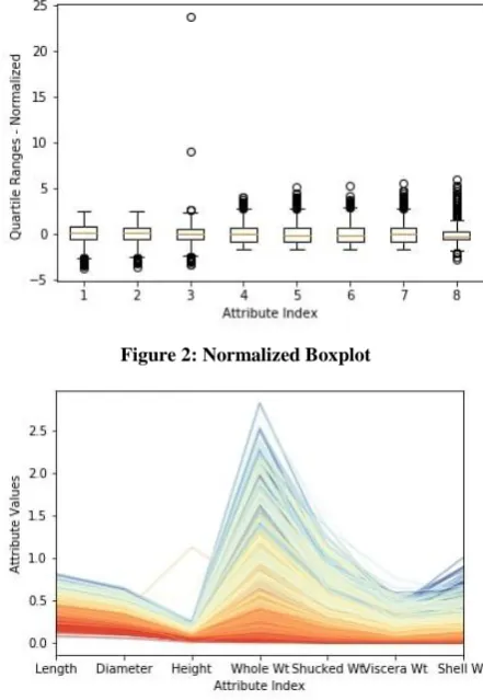
The minimum, maximum, mean, median, standard deviation and interquartile range of all the numeric attributes along with dependent variable of the dataset is calculated and plotted using a boxplot for easy visualisation of outliers. Due to the larger range of “Rings” variable, an unnormalized boxplot renders the other variables’ boxplots incomprehensible by squeezing their ranges. To bring all the variables on the same scale, they are normalized such that they all have zero mean and standard deviation 1. Figure 2 shows this boxplot. The attributes Length and Diameter have almost the same normalized range while there are a few outlying values for the Height attribute which might make the task of regression difficult. All the Weight attributes also have almost the same normalized range. The Rings label is not analyzed since it will be used in an unnormalized form for the regression to obtain a proper value of MAE.

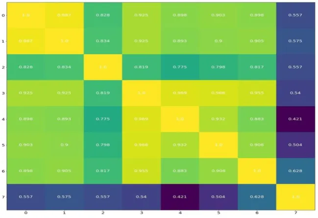
Next, the relation among the variables and between the variables and label is analyzed. The normalized attribute values for each example are first passed through a logit function to fit them in the range (0,1) which removes any negative values that may be there after normalization. A parallel plot (Figure 3) is constructed which plots these values of all attributes and it is coloured based on the value of the label (Rings). Dark brown represents less rings while dark blue represents higher number of rings. The parallel plot reveals significant correlation between each of the attributes and the label for each of the examples; similar colour shades are grouped together at several attributes for similar values.

This suggests that the prediction model will be fairly accurate. However, there are a few examples which do not follow the above trend. Dark blue lines mixed with lighter blue lines on the right and some blue lines in between the brown ones suggest these examples will be difficult to predict correctly.

Figure 2: Normalized Boxplot

Figure 3: Parallel plot

Figure 4: Annotated Correlation Heatmap

3.

LITERATURE REVIEW

The abalone dataset was first published in 1995. Since then, copious amounts of research using many different algorithms and methods has been done, first among them being decision trees. In 1999, CLOUDS, a decision tree based algorithm was used to achieve a 26.4% accuracy on the abalone test dataset. [6] Typically in classification problems, the algorithm for selecting a split point for the dataset at each internal node involves sorting the values of each numeric attribute, calculating the gini index (an evaluation metric for decision tree based classifiers) at each possible split point and selecting the split point with the minimum gini value. This brute force method was found to be computationally expensive and challenging [6]. Thus, CLOUDS used a better approach called SSE [6] in which the range of each attribute in the dataset was divided into intervals using quantiling techniques, an estimation of gini values at the boundaries of these intervals was made and compared with the minimum of the actual gini values at the boundaries. Thereafter, the brute force method was applied only in the intervals where the estimated gini value was less than the minimum gini value. This method was found to require at most only two read operations (opposed to the many needed for sorting technique implemented on smaller memories) on the dataset and was highly accurate in predicting the correct gini value as would be obtained by the brute force approach. However, using SSE did not lead to any significant improvement in classification accuracy or tree size for abalone dataset over the sorting technique, which obtained an accuracy of 26.3%[6]. C4.5 is another decision tree technique which achieved only 21.5% accuracy.[4]

K-means clustering algorithm run on a preprocessed dataset with reduced classes (8 classes), all numeric attributes and with one-fourth of the dataset left out for testing results in an accuracy of 61.78% [7] The experiment also helps in determining the relative contribution of different attributes to the classification accuracy (in increasing order of importance): Sex, Length, Height, Whole weight, Shell weight, Viscera weight, Diameter, Shucked weight. [7]

An Ordinary Least Squares (OLS) regression model that takes manipulated attributes as input for estimation of number of rings (and hence age) along with an ordered probit model for classification of the estimated value into three classes was

found to work well in classifying abalones with rings in the range of 3 to 14 for those three classes. However, the regressor was not accurate in its estimation. [2]

Neural networks, CasCor, CasPer and Conditional Generative Adversarial Networks (CGANs) have all been employed to solve the abalone problem too.[4] For all of these methods, the categorical attribute ‘Sex’ was converted into a numeric attribute in scale with the other attributes. A three layer neural network having eight units in input layer (one for each attribute), 29 units in the output layer (one for each class) and 1000 hidden units that uses Batch SGD for backpropagation and runs on a cross-validated dataset (divided in the ratio 6:2:2) obtained an accuracy of 25.99% on the test dataset.[4]

Cascade Correlation (CasCor) is a supervised learning architecture for neural networks that begins with a minimum number of units and automatically adds and trains new units individually. Thus, it has a dynamic topology. CasCor learns faster than traditional neural networks and does not require backpropagation. Moreover, since the input weights of a unit are frozen once it is added, it enables the CasCor network to incrementally detect more complex features. [8] Using this architecture with 100 hidden units (but a similar neural network), a classification accuracy of 24.43% was obtained on the abalone dataset which is a significant improvement on the 19.73% obtained using traditional neural network with the same number of hidden units. [4] Extrapolating the results, it can be safely concluded that using CasCor will show an improvement over an identical traditional neural network.

CasPer is an improvement over CasCor that solves its generalization problem and tendency to create large networks. This is done using different learning rates on different units and employing RPROP. Using just the RPROP gradient descent in CasPer as an improvisation, an accuracy of 30.78% was obtained with just 50 hidden units. [4]

is reached when G is able to replicate the training data and D always outputs ½, representing it is not sure about the origin of input data. CGAN is a conditional version of GAN which aims to build a generative model which can generate data conditioned on specified class labels. This is done by adding a condition as input to both G and D. [10]

Due to the skewed nature of the abalone dataset, many techniques have been used to augment the dataset and make it more evenly distributed. CGAN was used to condition GAN on the classes that have lesser examples in the abalone dataset possibly with the belief that the resulting overall increase in the number of instances will also prove advantageous. However, on training the mixed (original instances plus instances generated by CGAN) dataset consisting of 29000 examples by CasPer, it was found that accuracy actually dips to 16.29% on the test set. [4] It can be concluded here that since GANs have been proved to generate meaningful data [9] but not to remove noise [4] which is something that CasPer can do [4], the CGAN used may have amplified the noise in the original abalone dataset due to which the performance of CasPer decreased.

Other methods that have been used to remove the imbalance in the data distribution are Synthetic Minority Oversampling Technique (SMOTE) and Tomek links. In SMOTE, the minority class is oversampled by taking each minority class example and generating synthetic examples along the lines joining any or all of its k minority class nearest neighbours. [11] Tomek links is an undersampling method wherein two instances that belong to two different classes and are nearest neighbours of each other form a Tomek link. Based on what is required, either only the majority class sample or both samples of the link are removed. During research on combining both SMOTE and Tomek links, SVM was used as a binary classifier on a modified abalone dataset (with one class positive and all others negative). It was found that classification accuracy of SVM on the modified dataset after negative examples have been removed using Tomek links was 99.26% [12].

4.

METHODOLOGY

The first step towards applying linear regression to predict the age of the abalone was to numerically code the Sex variable in the dataset. For this, the following approach was undertaken:

1. Two new attributes were created in place of Sex. Let them be S1 and S2

2. The Sex value of each example was checked.

3. If it is Male, then S1 is equated to 1 and S2 to 0

4. If it is Female, then S1 is 0 and S2 is 1

5. If it is Indeterminate, both are kept 0. [12]

The attributes were not normalized before training because most of them distribute in the range (0,1). [5] Nonetheless, a dataset with normalized attributes was trained on the best performing linear regression model later to validate the claim. The label was never normalized as was done in Dataset Analysis to ensure proper calculation of MAE.

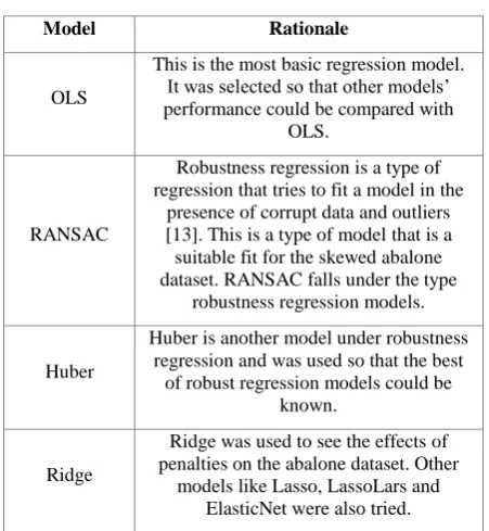
Table 2: Rationale behind model selection

Model Rationale

OLS

This is the most basic regression model. It was selected so that other models’ performance could be compared with

OLS.

RANSAC

Robustness regression is a type of regression that tries to fit a model in the

presence of corrupt data and outliers [13]. This is a type of model that is a suitable fit for the skewed abalone dataset. RANSAC falls under the type

robustness regression models.

Huber

Huber is another model under robustness regression and was used so that the best

of robust regression models could be known.

Ridge

Ridge was used to see the effects of penalties on the abalone dataset. Other

models like Lasso, LassoLars and ElasticNet were also tried.

Table 2 enlists the linear regression models selected along with the rationale behind the selection. All of these models were implemented using scikit library of Python.

All the models were run seven times till the performance no longer improved (with varied hyperparameters, where applicable) and the best performance of each model reported (in Table 3). For all of the models, techniques like SMOTE and 10-fold Cross-Validation were used to improve the quality of the dataset and the performance of the model. CGANs were not used to synthesize samples because the author believes that CGANs amplifies the noise in the dataset too which results in deterioration of performance.For the models without CV and without synthesized data, the dataset was divided in the ratio of 80:20 (in order) for training and testing purposes respectively. SMOTE has limitations due to which it cannot synthesize samples for labels having only one sample in the original data. Hence, examples having labels between 3 and 19 (including both) were synthesized (keeping the k_neighbours parameter 10 for better performance) and only labels within this range in the original as well as SMOTE data were used for training models. The data imbalance was removed by bringing the total examples for each label having less than 600 examples initially to 600 which is comparable to the majority class. The training and testing data was created with 80:20 ratio such that each class had approximately equal representation. 10-fold Cross Validation meant that the dataset was split in the ratio 90:10 and the reported error was averaged over the ten folds.

5.

RESULTS AND DISCUSSION

Table 3 lists the Mean Absolute Error for the various models with the corresponding hyperparameters in brackets, where applicable. The results for 10 fold CV have been averaged over the ten folds.

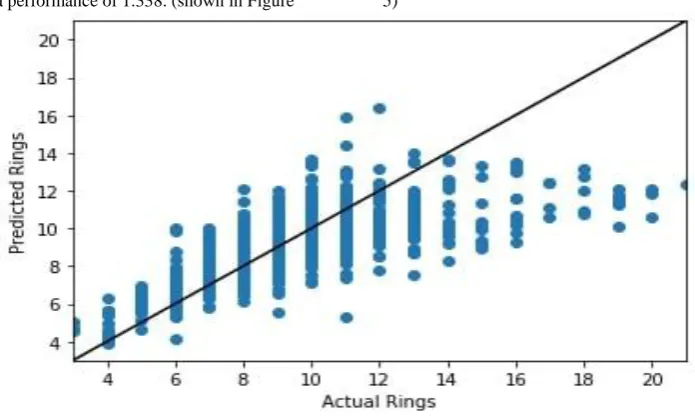
RANSAC yielded a performance of 1.338. (shown in Figure 5)

Figure 5: RANSAC on normalized dataset

Table 3: Results

Method Without SMOTE With SMOTE With 10 fold CV

OLS 1.500 1.875 1.636

RANSAC 1.332 (min_samples = 30) 1.830 (min_samples = 20) 1.583 (min_samples = 30)

Ridge 1.499 (alpha = 0.1) 1.882 (alpha = 0.01) 1.627 (alpha = 0.01)

Huber 1.399 (epsilon = 1) 1.885 (epsilon = 1) 1.605 (epsilon = 1)

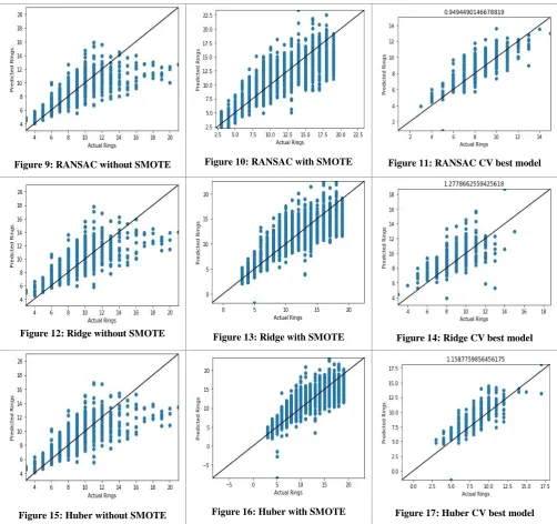
Table 4 shows the scatter plots of predicted rings versus actual rings for the various models and techniques used. Comparing Figures 6, 9, 12, and 15, it can be seen that the leftmost and rightmost points in OLS are a bit more spaced out than in Huber and RANSAC, with the points in RANSAC being the most condensed. Also, the scatter plot for Ridge is similar to the one for OLS. Even though RANSAC is the best performing model and it takes care of low-valued outliers, it still does not perform satisfactorily on the higher-valued outliers.

The scatter plots for SMOTE show points within the range which was selected for synthetic examples generation and there are visibly more points than in the corresponding scatter plots without SMOTE. Huber, Ridge and OLS seem to malfunction with all of them predicting negative number of

rings for a few examples. This may be due to the attributes of

the synthetic examples being weird. In comparison to the plots without SMOTE, the points in the plots with SMOTE are more vertically spread out.

The rightmost column of Table 4 shows the best model for each regression algorithm from among the ten models of the ten folds with the MAE for that model printed on top of the scatter plot. All of the models have a MAE around 1.0-1.1 which is significantly less than the best RANSAC model (1.332). However, these models represent only 10% of the data, have predictions having considerable difference from the actual value and may not generalize effectively. That being said, they do show the possibility of achieving a better performance.

Table 4: Scatter plot visualization of results

Figure 9: RANSAC without SMOTE Figure 10: RANSAC with SMOTE Figure 11: RANSAC CV best model

Figure 12: Ridge without SMOTE _{Figure 13: Ridge with SMOTE Figure 14: Ridge CV best model}

Figure 15: Huber without SMOTE Figure 16: Huber with SMOTE Figure 17: Huber CV best model

6.

CONCLUSION AND FUTURE WORK

In the task of predicting age of an abalone (by predicting number of rings) through its physical characteristics, the RANSAC regression model works best with a MAE of 1.332. Huber regressor does a pretty good job in comparison (MAE= 1.399) while penalized regression models cannot outperform OLS (MAE=1.5). All over, robustness regression models do a good job in dealing with outliers present in the abalone dataset.

Techniques such as SMOTE and Cross Validation do not improve the performance of the models with RANSAC performing the best here too achieving a MAE of 1.830. This cements its position as the best model. Normalization of attributes seems to result in the same performance as unnormalized data.

The scatter plots for individual folds of cross validations show that Mean Absolute Error can be brought down below 1 for certain arrangements of data, the best being 0.936. However,

it also shows that the error is still above the acceptable limits in some regions. It is the author’s belief that given an adequate and balanced dataset, RANSAC along with SMOTE and Cross Validation can achieve the goal of Mean Absolute Error less than 0.5 across all the labels.

7.

REFERENCES

[1] Abalone: https://en.wikipedia.org/wiki/Abalone

[2] Hossain, M, & Chowdhury, N (2019) Econometric Ways to Estimate the Age and Price of Abalone. Department of Economics, University of Nevada.

[3] UCI Machine Learning Repository, Abalone dataset: https://archive.ics.uci.edu/ml/datasets/Abalone

[5] Bowles, M (2015). Machine Learning in Python: Essential Techniques for Predictive Analysis, John Wiley & Sons, Inc.

[6] Alsabti, K., Ranka, S., & Singh, V (1999) CLOUDS: A decision tree classifier for large datasets.

[7] Mayukh, H. (2010) Age of Abalones using Physical Characteristics:A Classification Problem. Department of Electrical and Computer Engineering, University of Wisconsin-Madison.

[8] Fahlman, S & Lebiere, C (1990) The Cascade-Correlation Learning Architecture. Neural Information Processing Systems Conference, 1990.

[9] Goodfellow, I et al (2014) Generative Adversarial Nets. Department of Computer Science and Operations

Research, University of Montreal, Canada.

[10] Mirza, M (2014) Conditional Generative Adversarial Nets. Department of Computer Science and Operations Research, University of Montreal, Canada.

[11] Chawla, N. (2002) C4.5 and Imbalanced Data sets: Investigating the effect of sampling method, probabilistic estimate, and decision tree structure.

[12] Saina, H & Purnamia, S (2015). Combine Sampling Support Vector Machine for Imbalanced Data Classification, The Third Information Systems International Conference.