Multilayer Perceptron based Model of Large-Scale Gene
Regulatory Network
Taiwo Adigun
Department of Computer Science, University of Ibadan, Ibadan, Nigeria
Angela Makolo
Department of Computer Science, University of Ibadan, Ibadan, Nigeria
ABSTRACT
Background: The computational reconstruction of Gene Regulatory Networks (GRNs) using different techniques have encountered the challenge of constructing large network because of many parameters to be fitted and the nature of the input data. In fact, contemporary works on GRN inference that involve the use of hybridized techniques especially Artificial Neural Network (ANN) with meta-heuristic optimization techniques have to trade off computational cost for accuracy in reconstructing large-scale GRN. This work designed an efficient feature selection algorithm with GRN model to overcome the dimension problem of input data using biological prior knowledge of co-expression and network sparseness, so as to capture and represent the actual interrelationship among genes.
Methodology: The GRN model is an ensemble Multi-Layer Perceptron (MLP) network incorporating a novel feature selection algorithm termed Fuzzified Adjusted Rand Index (FARI). FARI is developed to investigate and establish the expression trends of genes in an expression profile data. A rank matrix of all genes produced by FARI shows their co-expression relationship, which is used to co-ordinate the selection of potential predictors as input features into the inference model. Each target gene is modeled separately by updating its parameters independently as several sub-problems of the overall network. The performance of the model is subjected to synthetic, ecoli and Mtb data.
Result: The result indicated an improved accuracy in the construction of large-scale GRN including a significant speed-up. The result on Mtb identified CCL5 as the first expressed gene, which is the same with CCL1 identified by the experimental method. Some of the expressed genes were validated through their biological pathways showing immune responses and host susceptibility to TB.
Conclusion: The included prior biological knowledge in MLP model provided the construction of an accurate large-scale GRN by reducing the potential large search space of GRN modeling. Besides, the model produced two major biological networks from the same process using the same dataset for appropriate biological validation.
Keywords
Gene Regulatory Network, Multi-Layer Perceptron, Fuzzified Adjusted Rand Index, prior knowledge, co-expression, rank matrix
1.
INTRODUCTION
A Gene Regulatory Network (GRN) is a collection of DNA segments in a cell which interact with each other indirectly (through their RNA and protein expression products) and with other substances in the cell to govern the gene expression levels of mRNA and proteins. The network structure is an abstraction of the system's chemical dynamics, describing the
manifold ways in which one substance affects all the others to which it is connected. The interrelationship of cell constituents govern the gene expression levels of mRNA and eventual production of proteins in the body, and this provides fruitful information on functional role of individual genes in a cell, and also helps to study dynamics of specific genes under particular diseases or experimental conditions. Genetic regulatory network consists of set of genes, proteins, small molecules, and their mutual regulatory interactions. In a cellular system, the functional role of individual genomic-encoded constituent is provided by the fundamental understanding depicted by GRN, which also help to identify the interactions between the constituents [1]. The development and functioning of organisms’ cell emerge from interactions in genetic regulatory networks [2]. The regulation of gene expression is achieved through the interactions between DNA, RNA, proteins, and small molecules. This regulatory system can be described by the structure of network called genetic regulatory network [3].
The reversed engineering of GRNs is from Microarray data because the pattern of expression profiles reflects the internal mechanism of gene interactions. The dataset can be a temporal or time-series data, which is in the form matrix of order N by M. N represents the number of genes and M represents length of experiments/time-points/samples. Apart from the fact that the gene expression dataset are complex, non-linear, dynamic and noisy; the number of genes (features) in a dataset is generally two or three times more than the number of experiments/time-points/samples. This imposes a well-known computational problem called curse of dimensionality especially when reconstructing large networks. Mores so, an important property of gene network is sparseness, which means that genes are regulated by a small constant number of other genes (i.e. 3-5 genes in bacteria). Hence, there is justification to prune the search space appropriately during network inference.
Many computational approaches have been developed for gene regulatory networks inference. Unfortunately, inference can be complicated if the amount of augmentation (parameters) is large [7]. Previous researches have shown that it is difficult to re-construct large-scale networks of GRN due to high dependencies among the parameters in large data, that is, there is need to balance between fitness value and the actual network structure of large scale networks [4]. This suggests that there has been a trade-off between accuracy and efficiency among GRN computational models. So, there is need for an effective model that would be able to handle the high dependencies among the parameters and the missing data which can cause the slow rate of convergence of NN inference.
The study is hinged on two recent reported works of Mandal et al. [4], and Raza and Alam [1]. Mandal et al. hybridized two meta-heuristic algorithms with RNN to reconstruct gene regulatory network but later concluded that they had to totally sacrifice computational cost for accuracy. They suggested the use of regularization method, inclusion of prior knowledge of GRNs and application of parallel computing method to improve the accuracy and speed of GRNs inference. Raza and Alam used extended Kalman Filter in back-propagation through time training algorithm with RNN for GRN inference, but later concluded that modeling a large scale GRN is still a challenge. They identify three problems with microarray data responsible for this challenge such as curse of dimensionality problem, inherent noise due to experimental limitations and data reliability. Now, this study addresses the challenge of reconstructing large-scale GRNs by tackling the problems identified by Raza and Alam using one of the approaches suggested by Mandal et al.
This work developed a novel feature selection algorithm using an improved Adjusted Rand Index (ARI), and biological prior knowledge of co-expression and network sparseness to deals with the dimension problem, which is the major hurdle to cross during GRN investigations. The result of the feature selection algorithm is a rank matrix, which serves two purposes; firstly, it is used to extract gene co-expression
modules for the construction of gene co-expression network. Besides, it is used to pick the appropriate features from the original dataset as the input into the training model instead of bombarding the model with the whole dataset. Section 2 of this paper discusses the theoretical background of major concepts while the details of the methods used to develop the GRN structure is discussed in section 3. The effectiveness of the proposed method is verified in section 4 by reporting different results and comparisons with other state-of-the-art methods. The paper is concluded in section 5 with recommendations.
2.
THEORETICAL BACKGROUND
The theoretical concepts of gene co-expression, Adjusted Rand Index (ARI) and MLP are provided here for better understanding of the methodology of this study.
2.1
Gene Co-expression
Gene expression is a biological process used by all living cells to generate the macromolecular machinery for living. It is the process by which information from a gene is used in the synthesis of a functional gene product (protein), which determines both the physical (phenotype) and disease traits of an organism. The interrelationship among genes in a cellular system is called Gene Co-expression Network (GCN) because genes of the same network are known to be either functionally related, controlled by the same transcriptional regulatory process or generally take part in a common biological process [18]. In a gene co-expression network, the genes signify a gene module and the edges indicate significant correlations [13]. Hence, a module is a set of genes with similar expression pattern in different samples of gene expression profiling. A module represents a highly connected sub-graph extracted from aco-expression network, which is a cluster of genes that have similar expression trends in different samples, but does not attempt to infer the causality relationship among the genes [18],[19].
Measuring expression trend is a process of computing association between a pair of genes that gives insight into whether they are co-expressed or not, which is central to the construction of both co-expression network and regulatory network. The expression trend of two genes exposes their pattern similarity, where co-expressed genes show their expression levels increasing or decreasing together under the same experimental conditions or time-points across the samples. Most of the existing methods are based on correlation measures and Mutual Information (MI), which uses global similarity to draw the relationship between genes but expression profiles share local similarity rather than global similarity [18]. MI leads to information loss due to the discretization of expression values and bi-clustering tends to be computationally expensive though suitable [18].
Figure 1: Expression patterns of two genes recA and uvrA in ecoli dataset having the same expression trend
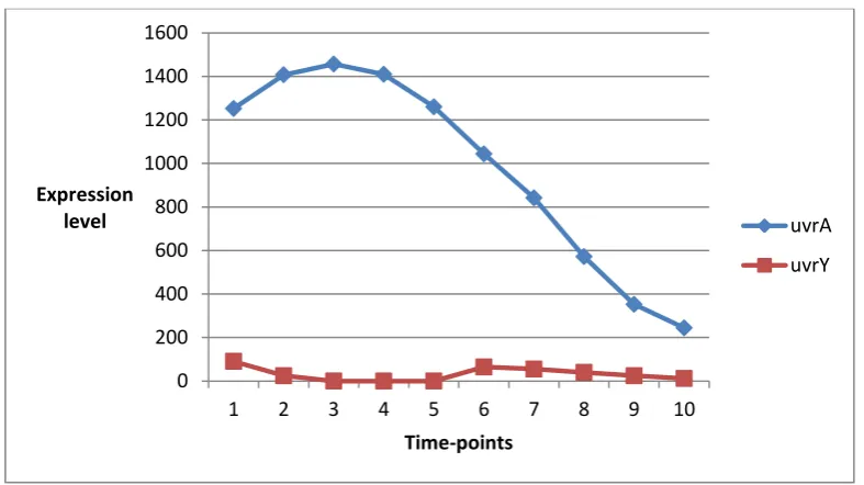
Figure 2: Expression patterns of two genes recA and uvrA in ecoli dataset having the different expression trend
Figure 3: Expression patterns of two genes recA and uvrA in ecoli dataset having the mixed expression trend 0
500 1000 1500 2000 2500
1 2 3 4 5 6 7 8 9 10
Expression level
Time-points
recA
uvrA
0 200 400 600 800 1000 1200 1400 1600
1 2 3 4 5 6 7 8 9 10
Expression level
Time-points
uvrA
uvrY
0 200 400 600 800 1000 1200 1400 1600
1 2 3 4 5 6 7 8 9 10
Expression level
Time-points
uvrA
[image:3.595.116.480.551.742.2]2.2
Adjusted Rand Index
Adjusted Rand Index is an adjustment to the ordinary Rand Index to account for agreement by chance. Rand Index is a metric proposed by [25] for measuring the agreement between two clustering solutions. It gives a value between 0 and 1, with 0 representing little agreement and 1 representing strong agreement. A good measure of agreement is needed to compare clustering results especially against external criteria. Adjusted Rand Index is a measure of correspondence between two partitions of the same data and is based on how pairs of objects are classified in a contingency table. It returns a single value indicating the level of agreement between two partitions. An ARI score of 1 indicates that the two clustering results are the same while 0 indicates that the two clustering results are not the same. However, the value of Adjusted Rand Index can be negative, corresponding to very low agreement, but cannot be greater than 1. Adjusted Rand Index was used by Santos and Embrechts [20] as a feature selection method because the measure of agreement between partitions and the target data is partitioned by means of the labeling. This is done by splitting each feature in non-overlapping equal intervals and compares the partition derived from the split with the one given by the targets. By doing this each feature's discriminant power is being evaluated and the features ranked according to the computed ARI value. The most discriminant features is then selected and applied in the classification algorithm.
[image:4.595.312.546.140.436.2]Computing ARI starts by building the Contingency Table (similar to confusion matrix) for the two clusters. The contingency table is filled in by calculating the size of intersection of each group in the clusters against each other, which is formed by the number of items that are either in agreement or disagreement in the groups of the two clusters. According to [20] and [22], contingency table is described as follow; consider a set of n objects S = {O1,O2 ……On} and suppose that U ={u1; u2 …. uR} and V = {v1, v2, ….. vC} represent two different partitions of the objects in S such that URi=1 ui = S = UCj=1vj and ui ∩ ui, ɸ = vj ∩ vj, for 1≤ i ≠ i’ ≤ R and 1 ≤ j ≠j’ ≤ C. Given two partitions, U and V, with R and C subsets, respectively, the contingency Table 1 can be formed to indicate group overlap between U and V. The Table below can be formed to indicate group overlap between U and V.
Table 1: Contingency Table for Comparing Partitions U and V
Partition
V
Group v1 v2 …. vC Total
U
u1 t11 t12 …. t1C t1.
u2 t21 t22 …. t2.
. . .
. . .
. . .
. . .
. . .
. . .
uR tR1 tR2 …. tRC tR.
Total t.1 t.2 …. t.c t.. = n
In the table above, trc, represents the number of objects that were classified in the rth subset of partition R and in the cth subset of partition C. From the total number of possible
combinations of pairs of objects from a given set we can represent the results in four different types of pairs:
a - objects in a pair are placed in the same group in U and in the same group in V;
b - objects in a pair are placed in the same group in U and in different groups in V ;
c - objects in a pair are placed in the same group in V and in different groups in U and;
d - objects in a pair are placed in different groups in U and in different groups in V .
This leads to an alternative representation of Table 1 as a 2 X 2 contingency table (Table 2) based on a, b, c, and d.
Table 2: Simplified 2 X 2 Contingency Table for Comparing Partitions U and V.
Partition V
U Pair in same
group
Pairs in different groups
Pair in same group a b
Pairs in different
groups c d
ARI is given as:
adjustedRandIndex(x,y)=
(1) where
Index, MaxIndex and ExpectedIndex are calculated from the contingency table built from the two clusters.
2.3
Multilayer Perceptron (MLP)
MLP is a Feedforward Neural Networks (FNN), which is the most popular and most widely used models in many practical applications [9],[12],[15]. An FNN is an NN where connections between the units do not form a directed cycle. The FNNs were the first and arguably simplest type of NN devised. In this network, the information moves in unidirectional connection between the neurons whereas different connectivities yield different network behaviours. Generally, FNN are static, which produce only one set of output values rather than a sequence of values from a given input. FNN are memory-less whereas their response to an input is independent of the previous network state. There are no cycles or loops in the network like Recurrent Neural Networks. A typical FNN consists of layers. The input layer followed by a hidden layer, which consists of any number of neurons, or hidden units placed in parallel and an output layer of neurons. Each neuron performs a weighted summation of the inputs, which later on is passes through a nonlinear activation function.
It is a finite, directed acyclic graph, which extends the perceptron with hidden layers of processing elements. It directly incorporates the capabilities of higher order networks but using a larger number of weights and processing units. The resulting map is very flexible and powerful, but it is hard to analyze, exhibits slower learning, and is vulnerable to incremental addition of units. However, this model is
Index – ExpectedIndex
[image:4.595.50.285.540.707.2]systematically designed with a powerful feature selection algorithm to eliminate these limitations in building biological large networks. The MLP constructs input-output maps that are nested composition of non-linear functions.
3.
METHOD
3.1
Fuzzified Adjusted Rand Index (FARI)
Building contingency table is central to the use of ARI, which is formed by the number of items that are either in agreement in the groups of the two clusters. However, it is impractical to get the measure of agreement of gene expression values because they are usually real values. Fuzzy concept of rule sets is incorporated in the process of building the contingency table, and this is the point of improvement of the research work.ARI is given as:
adjustedRandIndex(x, y) =
where
Index, MaxIndex and ExpectedIndex are calculated from the contingency table built from the two clusters
- [
]/
½[ ] - [ ]
(2) Where nij, ai, bj and n are values from the contingency table FARI gives an insight into the relationship between genes, which eventually gives the opportunity to pick the most plausible genes as the best combination of affecting/regulatory genes unlike creating hypothetical connections by using conditional combinations of gene as input in [4] or using constraint to prune the network in [10] and [1]. By using FARI, each gene sample discriminant power
is being evaluated and the genes are ranked according to the computed ARI values while making connection between the curse of dimensionality and sparseness property of biological network.
3.2
Contingency Table Algorithm
The building of contingency table is very central to the use of adjusted rank index because all the values used in the calculation of the adjusted rand index are taken from the contingency table. A contingency table is a tabular form of relationship between variables filled in with integer numbers, which shows the level of agreement or disagreement among the categorical variables of the two clusters.
Given a set S of n elements, and two groupings or partitions (clusters) of these points, i.e
X = {x1, x2, ………., xr}
Y = {y1, y2, ………., ys}
The overlap/intersection between X and Y can be summarized in a contingency table nij, each entry nij denotes the number of objects in common between Xi and Yj.
i.e nij = |Xi∩Yj|
The overlap is a measure of proximity between a pair of genes across samples, showing the transcript levels of two co-expressed genes rising and falling together. Since gene expression data are real values; hence, it is difficult to calculate number of common objects in two gene sample profiles. Fuzzy rules concept is applied to eliminate this challenge, where levels of agreement of samples of a gene against other samples of the other gene are distributed into different bins and clusters. Different values (measures) representing class labels are attached to bins and clusters accordingly. Each value is then used to fill contingency table of two gene objects of different samples.
3.3
Building of Fuzzy Rules
The process of separating data into groups according to their respective class labels, which is the first step in fuzzy rule generation is perform by applying two conditions. The conditions are whether the two samples between a pair of genes are the same time-point or not. The first condition separates data into discrete interval (bins), while the second condition separates the data into clusters.
Given a pair of genes X and Y and the expression values rescaled to interval [0, 1] by use of a linear transformation;
i. The first condition checks similar expression pattern of two samples Xi and Yi. This is at the same experimental condition or time point (i.e local similarity)
Let Xp and Yp be expression patterns of genes X and Y at point i, we have two discrete values as class labels nij = 10 and nij = 0.
The membership function, which is the first step in fuzzy rule generation of these groups is constructed as follow:
Xp = exp(Xi – Xi-1) (3) Yp = exp(Yi – Yi-1)
(4)
If (Xp>0 and Yp>0) OR (Xp<0 and Yp<0) Then nij = 10 ---> bin 1 Else,
nij = 0 ---> bin 2 where Xi-1 = 0.0 if i = 1
The intuition behind this partitioning follows the principle used in filling the contingency table of ARI, where the values of the table determined the level of similarity of two clustering results across groups. Bin1 represents the situation where the expression trends of two genes are the same at the same time-point or experimental condition, while Bin2 represents situation where two genes have different expression trends.
ii. The second conditions checks similar expression pattern of two samples Xi and Yj when i≠j. other similarity across samples (i.e global similarity). Let AD be the absolute difference (AD) of expression values of genes X and Y at Xi and Yj when i≠j being the size of their intersection, the values of the intersection are partitioned into six (6) different clusters as the class label using integer values, scale = [5, 4, 3, 2, 1, 0].
The membership function is constructed as follow; Index – ExpectedIndex
MaxIndex - ExpectedIndex
AD = exp(|Xi – Yj|) (5)
The data point clusters are defined by AD as follow; Data-points nij Clusters
0.00 – 0.049 5 Cluster 1
0.05 – 0.09 4 Cluster 2
0.10 – 0.19 3 Cluster 3
0.20 – 0.349 2 Cluster 4
0.35 – 0.49 1 Cluster 5
0.50 – 1.00 0 Cluster 6
The AD partitioning into data points also follows the principle of filling of contingency table of ARI. The values assigned to each partition shows the measure of agreement or disagreement between gene expression values, where the highest value indicates relatedness and lower value indicates disagreement. The ranges of partitions are assumed between 0 and 1 because the original gene expression data has been normalized between 0 and 1.
Existing techniques generally depend on proximity measures based on global similarity to draw the relationship between genes, but it is observed that expression profiles share local rather that global similarity [18].
3.4
MLP Based GRN Model
The use of MLP for GRN model inference is based on the assumption that the regulatory interactions between genes can be represented in the form of a neural network where nodes are the genes and the edges define the nature of regulatory interaction. With time-series expression dataset, the output of a gene node of time ‘t+Δt’ may be calculated from expression values and connection weights of plausible genes selected by the ranking given by the feature selection algorithm at time ‘t’.
An ensemble of feed forward multilayer perceptron of total genes n is adopted for the whole network inference where the architecture of each member of the ensemble is a MLP (decouple network) for each gene modeling with different four layers;
One (1) input layer with l units of neurons, l is the number of highly ranked genes against the target gene.
Two (2) hidden layers with k units of neurons in the first layer h and q units of neuron in the second layer g.
One (1) output layer with one neuron of the calculated expression value of the target gene at ‘t+∆t’
The model equation at any neuron is given as: ei(‘t+Δt’) = f(∑ej(t)wij + bi), j =1-n (7) where
ei is the expression level of gene i (1≤i≤n), n is the total number of genes,
wij is the synaptic weights representing the regulatory effect of gene j on gene i (1≤i, j≤n). A positive value of synaptic weight wij indicate
activation of gene j on gene i, a negative value indicate inhibition and wij = 0 means that gene j has no regulatory effect on gene i.
f(.) is a non-linear transfer function, which is sigmoid function
f(u) = 1/(1+exp(u)) (8)
The MLP formalism and modeling involves updating set of parameters wij and bi, which were initialized as;
wij = 0 bi = 0.001
The nature of the value of wij has biological significance whether wij<0, 0 or >0. Hence, regulatory effect of a gene is taken to be the updated weights of all genes connected to the gene.
The parameters of the MLP layout of each ensemble are given as:
Wkl = weights associated with the links between the input layer and h
Vqk = weights associated with the links between h and g
Uiq = weights associated with the links between the output layer and g
Eventually, the MLP constructs input-output maps that are a nested composition of non-linarites. Based on the two hidden layers;
ei = f(∑uiq.f(∑vqk.f(∑wkl.ej +bl) +bq) +bi) (9)
Each member of the ensemble is a multivariable regressor (many-to-one) trained with gene expression matrix data to learn correlations of descriptor genes with the target gene. Once the ensemble network is built, the connection weights determine the topology of the regulatory network.
3.5
Learning Rule – Gradient Descent
Optimization with Back-propagation
Gradient descent is an important local optimization algorithm and back-propagation trains a feed-forward multilayer neural network for a given set of input patterns. Gradient Descent is an iterative minimization method, which shows the direction of the steepest ascent of the error function. The network examines its output response to the sample input pattern and compares the output with the desired output to calculate the error value.yji = f(∑k=1y(j-1)wjik) (10) yji = output from the j-th neuron in layer i
wjik = connection weight from the k-th neuron from layer (j-1) to the i-th neuron in layer j
f(x) = 1/(1+exp(-x)) (11)
ep = ∑p ∑i(dji - yji)2 (12) ep = MSE of output errors for every training sample pattern
dji = desired output from the i-th neuron in layer j With GD, the weight change can be performed as:
∆wt = -η(δep(w)T
/ δw) (14)
η = scaling factor/learning rate δep(w)T
= first derivative of the logistic function
3.6
Network Performance Metrics
The validation of the proposed method is measured in terms of correct prediction of regulations in the GRN, which is used to evaluate the performance of the network inference method. The metrics for the evaluation are sensitivity (Sn), specificity (Sp), accuracy and Matthew’s correlation coefficient (MCC). They are defined as follows:
Sn = TP/(TP+FN) (15)
Sp = TN/(TN+FP) (16)
Accuracy = (TP+TN)/(TP+TN+FP+FN)
(17)
MCC=((TP*TN)-(FP*FN))/√((TP+FP)*(TP+FN)*(TN+FP)*(TN+FN)(18)
TP (True Positive) = number of correctly predicted regulations (both activations and inhibitions). TN (True Negative) = number of correctly predicted non-regulations (zero weights).
FP (False Positive) = number of incorrectly predicted regulations.
FN (False Negative) = number of incorrectly predicted non-regulations
4.
IMPLEMENTATION
All the implementations were performed using Python programming language on Ubuntu Linux 14.0.4 platform, executed on AMD 1.30Ghz processor and 2GB of RAM.
5.
RESULTS AND DISCUSSION
5.1
Results of Artificial Dataset
The ultimate of this study is to reconstruct a large-scale GRN that will balance between the fitness value and actual network structure. Modeling a GRN that will maintain prediction performance as the network complexity grows has been a
challenge, which [1] submitted that curse of dimensionality problem and inherent noise of the experimental data are major issues of the challenge. Incidentally, [4] suggested inclusion of prior knowledge of GRNs as one of the major ways to improve accuracy and speed of a large-scale GRN. FARI is developed to tackle the curse of dimensionality problem and noisy data using prior knowledge of co-expression and sparseness of biological networks to improve the prediction performance of large-scale networks with good speed. The data gotten from [4] contains 30 genes with 50 data-points in 5 datasets making it to be 250 data-data-points altogether. A discretized weight matrix of 30x30 dimension is then generated, with zeros representing regulations and non-zeros representing regulations (-1 as inhibition and 1 as activation).
There are 72 non-zero values of weights defining the number of regulations and 828 zero values, from which the performance of the model is analyzed. The zero values include the non-existence edges that were not selected for the training by the feature selection algorithm. False regulations and non-regulations come from training set that could not meet the minimum fitness value at 1000th iteration and the ones that meet the minimum fitness value beyond 600th iteration because majority of the decoupled network achieved the optimum fitness value between 108th and 380th iteration. The correctly predicted regulations are eventually used to construct the GRN.
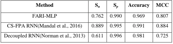
[image:7.595.151.445.551.626.2]Correctly predicted regulations (TP) = 64 Incorrectly predicted regulations (FP) = 8 Correctly predicted non-regulations (TN) = 808 Incorrectly predicted non-regulations (FN) = 20 The overall execution time of the ensemble network is at the average of 40mins against 1.5hours recorded by Mandal et al. using the same dataset. Table 4.10 shows the performance and comparison of this model with the reported result from [4] on the artificial dataset in terms of Sensitivity (Sn), Specificity (Sp), Accuracy and Matthews Correlation Coefficient (MCC).
Table 3: Performance Analysis and Comparison of the Constructed GRN
Method Sn Sp Accuracy MCC
FARI-MLP 0.762 0.990 0.969 0.807
Figure 5: Performance Analysis of the GRN Model
5.2
Evaluation Results of Real Data of SOS
DNA Repair Networks
[image:8.595.36.301.394.522.2]The reconstruction of GRN from a real dataset of SOS DNA repair network of e.coli is on experimental dataset described by [4] and [1] contains expression of 8 major genes due to their significant involvement in the process of DNA repair. The genes under consideration are UvrD, lexA, umuD, recA, uvA, uvrY, ruvA and PolB with 50 time-points, and the values are normalized in the range of [0,1].
Table 4: Weight Matrix of e.coli showing Regulations and Non-regulations
uvrD lexA umuDC recA uvrA uvrY ruvA polB
uvrD 0 0 0 0 0 0 0 -2
lexA 0 0 0 0 0 0 0 -2
umuDC 0 0 0 1 0 0 0 -1
recA 0 1 0 0 1 0 0 -2
uvrA 0 1 0 0 0 0 0 -2
uvrY -1 0 0 0 0 0 0 -2
ruvA 0 0 0 0 0 0 0 0
polB 0 0 0 0 1 0 0 0
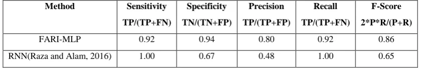
Model parameters chosen for e.coli GRN include Sigmoid transfer function, initial weights equal zeros, and the input value n = 4 is used as the hypothetical regulators because e.coli is a small cell. We generated a discretized weight matrix of 8x8 (Table 4) showing the regulations (activations and inhibitions) and non-regulations, from which the GRN is constructed and transcription factors identified. Performance analysis of the model on e.coli SOS DNA repair data is shown in Table 5, including the comparison with the result reported by [1] on the same dataset. It can be observed that the performance metrics are good representations of a better model even when compared with the work of [1]. There are 12 interactions that are correctly predicted shown in Table 4 and a clear cut discovery is made where polB gene happens to inhibit almost all other genes, whereas lexA gene has been reported to inhibit all other genes in e.coli SOS DNA repair network. This discovery is queried by searching the e.coli SOS DNA repair network genes on KEGG database (https://www.genome.jp/kegg/pathway.html ) and we discovered that polB gene engages in more pathway networks than all other genes. This discovery is subject to further experimental verifications and analysis.
Table 5: Performance Analysis and Comparison of the Model on e.coli
Method Sensitivity
TP/(TP+FN)
Specificity TN/(TN+FP)
Precision TP/(TP+FP)
Recall TP/(TP+FN)
F-Score 2*P*R/(P+R)
FARI-MLP 0.92 0.94 0.80 0.92 0.86
RNN(Raza and Alam, 2016) 1.00 0.67 0.48 1.00 0.65
0 0.2 0.4 0.6 0.8 1 1.2
Sn Sp Accuracy MCC
FARI-MLP
Mandal et al.(2016)
[image:8.595.88.515.553.623.2]Figure.6: Performance Analysis on e.coli Data
5.3
Results of Mtb-Stimulated Human
Macrophages Data
The model was also applied to Mtb data at latent stage to unfold the genes that are expressed and their transcription factors (TFs) in human during the latent stage of tuberculosis infection by reconstructing GRN. The first 1,000 genes of Mtb-Stimulated human macrophages data (GSE11199) generated by [21] are investigated, and the number of input genes of the MLP is set to eight (8) being a eukaryotic system. Out of the 1,000 gene set, 203 interactions were discovered from the gene regulatory network, where 177 genes were repressed and 26 genes were expressed (activated). The expressed genes are selected and further analyzed using KEGG database. Some of the expressed genes were found to be involved in one or two pathways while were not found in the KEGG database. The genes that involved in special pathways characteristics of immune responses especially in human macrophage, epithelial and dendritic cells, and susceptibility to tuberculosis. All these pathways play important roles in the latency stage of Mtb infection in human. Thuong et al. [21] identified CCL1 as a gene involved in host susceptibility to TB, whereas the computational model identified CCL5 among others. Both CCL1 and CCL5 have been observed to perform the same function, which is described to be C-C motif chemokine ligand by g:profiler (https://biit.cs.ut.ee/gprofiler/gconvert.cgi)
6.
CONCLUSION
In this work, a novel feature selection algorithm has been developed for the extraction of co-expressed genes using Adjusted Rand Index with Fuzzy rules. The new feature extraction model, Fuzzified Adjusted Rand Index (FARI) is used in conjunction with Multi-layer perceptron to reconstruct large Gene Regulatory Network (GRN). FARI has given an insight into the relationship between genes, which eventually gives us the opportunity to pick the most plausible genes as the best combination of affecting/regulatory genes in constructing gene regulatory network unlike creating hypothetical connections by using conditional combinations of gene as input or using constraint to prune the network in the previous works. This computational model eliminates difficulties encountered in re-constructing large-scale networks due to high dependencies among the parameters in large data. The balance between fitness value and the actual network structure of large scale networks is enhanced and overcomes the limitation of trade-off between accuracy and efficiency among GRN computational models. FARI
therefore uses the biological prior information to reduce the large search space created from the complex units of Multi-layer perceptron due to the complex nature of the input data. It was noted that ranking of genes to analyze their expression trends by FARI could be parallelized because it is done in pairs. Incorporating parallelism into the feature selection algorithm would further reduce the computational cost of the whole model. Besides, using neural network as the inference technique of GRN reconstruction involve the use of the weight matrix to describe the nature of the regulation, that can never be stable with the use of random numbers as the initial weights. It would be interesting to study the effect of random numbers as initial weights on the outcome of the inference using different ANN models.
7.
REFERENCES
[1]. Raza K. and Alam M.(2016) Recurrent Neural Network Based Hybrid Model of Gene Regulatory Network. Computational Biology and Chemistry, 64:322-334. [2]. Hidde, D.J. (2002) Modeling and Simulation of Genetic
Regulatory Systems: A Literature Review. Journal of Computational Biology, 9(9), 67-103.
[3]. Ji, R., Liu, D. and Zhang, W. (2010).The Application of Hidden Markov Model in Building Genetic Regulatory Network. J. Biomedical Science and Engineering,3, 633-637, doi:10.4236/jbise.2010.36086
[4]. Mandal S., Khan A., Saha G., and Pal R.K.(2016) Large-Scale Recurrent Neural Network Based Modelling of Gene Regulatory Network Using Cuckoo Search-Flower Pollination Algorithm. Advances in Bioinformatics Volume 2016, Article ID 5283937, 9 pages
[5]. Bower, J. (2001) Computational Modelling of
Genetic and Biochemical Networks. MIT Press, Cambridge.
[6]. Ching, W., Fung, E., Ng, M. and Akustu, T. (2005) On Construction of Stochastic Genetic Networks Based on Gene Expression Sequences. International Journal of Neural Systems, 15(4), 297-310.
[7]. Golightly, A. And Wilkinson, D.J. (2006) Bayesian Sequential Inference for Stochastic Kinetic Biochemical Network Models. Journal of Computational Biology Volume 13, Number 3, Mary Ann Liebert, Inc. Pp. 838– 851
0 0.2 0.4 0.6 0.8 1
FARI-MLP
[8]. Goutsias, H. and Lee, N.H.(2007) Computational and Experimental Approaches for Modeling Gene Regulatory Networks. Curr. Pharm. Design, 13(14):1415–1436. [9]. Gowri, T. M., and Reddy, V. V. C. (2008). Load
Forecasting by a Novel Technique using ANN. ARPN Journal of Engineering and Applied Sciences, 3 (2), pp. 19-25.
[10].Grimaldi, M., Visintainer, R. and Jurman, G. (2011).RegnANN: Reverse Engineering Gene Networks Using Artificial Neural Networks. PLoS ONE, Vol. 6, Issue 12, e28646.
[11].Hartemink, A., Gifford, D., Jaakkola, T., et al. (2002) Bayesian Methods for Elucidating Genetic Regulatory Networks. IEEE Intelligent Systems, 17(2), 37-43.
[12].Isa, N. A. M., & Mamat, W. M. F. W. (2011). Clustered-Hybrid Multilayer Perceptron Network for Pattern Recognition Application. Applied Soft Computing, 11 pp. 1457-1466.
[13].Jiang J., Sun X., Wu W., Li L., Wu H., Zhang L., Yu G. and Li Y. (2016). Construction and application of a co-expression network in Mycobacterium tuberculosis. Scientific Reports | 6:28422 | DOI: 10.1038/srep28422 [14].Khan A., Mandal S., Pal R.K. and Saha G.(2016)
Construction of Gene Regulatory Networks Using Recurrent Neural Networks and Swarm Intelligence. Scientifica Volume 2016, Article ID 1060843, 14 pages [15].Li, H., and Adali, T. (2008). Complex-Valued Adaptive
Signal Processing using Nonlinear Functions. EURASIP Journal on Advances in Signal Processing, pp. 1-9. [16].Mandal S., Saha G. and Pal R.K.(2017) Recurrent Neural
Network Based Modeling of Gene Regulatory Network Using Bat Algorithm.
[17].Noman N., Palafox L., and Iba H., (2013)“Reconstruction of gene regulatory networks from gene expression data using decoupled recurrent neural network model,” in Natural Computing and Beyond: Winter School Hakodate 2011, Hakodate, Japan, March 2011 and 6th International Workshop on Natural
Computing, Tokyo, Japan, March 2012, Proceedings, vol. 6 of Proceedings in Information and Communications Technology, pp. 93–103, Springer, Berlin, Germany, 2013.
[18].Roy S., Bhattacharyya D.K., and Kalita J.K.(2014). Reconstruction of gene co-expression network from microarray data using local expression patterns. BMC Bioinformatics 2014, 15(Suppl 7):S10
[19].Ruan J., Dean A.K., and Zhang W.(2010). A general co-expression network-based approach to gene co-expression analysis: comparison and applications. BMC Systems Biology 2010, 4:8
[20].Santos J.M., Embrechts M. (2009) On the Use of the Adjusted Rand Index as a Metric for Evaluating Supervised Classification. In: Alippi C., Polycarpou M., Panayiotou C., Ellinas G. (eds) Artificial Neural Networks – ICANN 2009. ICANN 2009. Lecture Notes in Computer Science, vol 5769. Springer, Berlin, Heidelberg.
[21].Thuong, N. T. T., Dunstan, S. J., Chau, T. T. H., Thorsson, V., Simmons, C. P., etal. (2008) Identification of Tuberculosis Susceptibility Genes with Human Macrophage Gene Expression Profiles. PLoSPathog4(12):e1000229.
doi:10.1371/journal.ppat.1000229
[22].Yeung, K. Y. and Ruzzo, W. L. (2001) Principal component analysis for clustering gene expression data. BIOINFORMATICS, Vol. 17 no. 9, Pages 763–774. [23].Zhang, S.-Q., Ching, W.-K. and Yue, J. (2008)
Construction and Control of Genetic Regulatory Networks: A Multivariate Markov Chain Approach. Journal of Biomedical Science and Engineering, 1, 15-21.
[24].Zhang, Z.-F. (2004) Constructing and Predicting Gene Regulatory Network Using Micro-Array Data. National Central University, Taiwan.