Performance Evaluation of Adaptive Signal Processing
Techniques in Reservoir Bathymetry Data
M. Selva Balan
Research Scholar,
DIAT, Pune
Scientist D,
CWPRS, Pune
C. R. S. Kumar
Associate Professor,
Department of Computer Engineering,
DIAT, Pune
ABSTRACT
Analysis of underwater bathymetry data using single-beam and multi-beam echo sounders has been recognized as an effective tool in estimation of sedimentation in a reservoir. However, the accuracy of sediment volume calculation depends on the quality of the backscatter data, received from the echo sounder. The echo signal reflection is sensitive to physical properties of medium, submerged vegetation and sediment characteristics. In this paper a novel approach is made by applying different gridding and signal processing techniques on a backscattered echo signal acquired form a natural lake formed in the western guards. This lake is selected as it is naturally formed with lots of sediment inflow due to change in agricultural practices. The data used for this study was collected at regular interval (i.e. 2003, 2013 and 2016). Data of 2003 and 2013 were used as input data and the performance validation was carried out in comparison with 2016 data, which is measured with the highest precession technology (i.e. RTK-DGPS) after completion the dredging process. The standard tools estimating the bathymetry suffers lack of adaptive modern filter capacities and hence results in erroneous depth measurement, which in turn leads to underestimation or overestimation of the capacity. The most advanced adaptive filters are applied on this lake data, and their performance was compared with reference to 2016 capacity estimation.
General Terms
Signal Processing, Reservoir Sedimentation, Computational Mathematics, Graphics and Imaging
Keywords
Bathymetry, Underwater Acoustics, Savitzky Golay, Wiener Filter, Signal Processing.
1.
INTRODUCTION
Modern multi frequency echo sounders provide substantial signal processing capabilities to mitigate the underwater channel fluctuations; however, these capabilities are extremely sensitive to the error in the estimation of the underwater channel characteristics (Fernandes, Chakraborty, & William, 2012).When an ultrasonic wave is transmitted through water, it is expected to reach the bottom and then reflect back, but instead of this, it gets added with noise and reflected back by the obstacles such as stones, underwater vegetation or the creatures living under the water. This gives a false bottom anticipation which results in error in the volume calculations.
In active sonar systems a short duration probing signal (in the millisecond range) is transmitted at a known time, which travels through the water column, and generates an echo when reflected from the water surface or from the bottom. Echo
signal strength at the receiver with grazing angle θ depends on three main components: Transmission Loss (TL), Target Strength (TS). Equation (1) presents the basic equation of active sonar.
𝐸𝐿 𝜃 = 𝑆𝐿 𝜃 − 2𝑇𝐿 + 𝑇𝑆 𝜃 (1)
Source Level (SL) typical value is 214dB (+/- 6dB) for SBES and for side scan sonar the typical value is 225 dB at 100 kHz. The transmission loss is dependent on the distance and frequency. The shallow water channels, particularly are characterized by multiple surface and bottom reflections so the transmission losses dominant. Transmission loss can be estimated by adding the effects of geometrical spreading, absorption and scattering. Acoustic signals in shallow water propagate within a cylinder bounded by the surface and the bottom, as a result cylindrical spreading appears. Transmission loss (dB) caused by cylindrical spreading is given by equation (2)
𝑇𝐿 = 10 log 𝑟 + 𝛼𝑟 × 10−3 (2)
Where∝ is absorption coefficient in dB/km and r is the range in meters. Transmission loss due to bottom reflection is as given in equation (3),
𝑇𝐿_𝐵𝑅 = 10 log 𝑚𝑠𝑖𝑛𝜃 −(𝑛2−𝑐𝑜𝑠2𝜃 )0.5
𝑚𝑠𝑖𝑛𝜃 +(𝑛2−𝑐𝑜𝑠2𝜃 )0.5
2
(3)
Wherem is the ratio of water density to sediment density and n is ratio of water sound speed to sediment sound speed. The other major factors that contribute to strength of echo signal are target strength as presented in equation (4), which is a function of backscatter strength BS at grazing angle θ and the area ensonified 𝐴𝑓, by a single beam of echo-sounder.
𝑇𝑆 𝜃 = 𝐵𝑆 𝜃 + 10 log 𝐴𝑓 𝜃 (4) Transmitting signal considering water as a channel is a challenge because of the effect of spreading, reverberation, attenuation and absorption adding to contribution due to ambient noises.The sources of ambient noise are both natural and machine made, with different sources exhibiting different directional and spectral characteristics (Jarrot, Ioana, & Quinquis, 2005). Therefore, before recognizing the received acoustic signal, it is necessary to remove the noise so as to keep the important signal features as much as possible.Based on spectral characteristics, ambient noise is made up of 3 constituent types – wideband continuous noise, impulsive noise and tonal noise.
International Journal of Computer Applications (0975 – 8887) Volume 180 – No.33, April 2018
relative to the reference level of 1 micro Pascal (µPa). Tonal noise is narrowband signal characterized as the amplitude in dB ref. 1µPa and frequency.
Based on sources, the main categories of noise include:
A. Hydrodynamic Noise: This type of noise is caused by the movement of water due to tides, winds, currents and storms. Level of hydrodynamic noise can be related to the condition of the surface of the water body. When the surface is agitated by wind or storm, the noise level increases which reduces the capability of detection (Sadaf, Yashaswini, Halagur, Khan, & Rangaswamy, 2015)
B. Seismic Noise: It is caused by movements of land under or near the sea (for example, during an earthquake). They are rare and also of short duration. (Sadaf, Yashaswini, Halagur, Khan, & Rangaswamy, 2015)
C. Biological noise: It is the result of a number of sources like marine animals, distance shipping, rain, wind, bubbles.
Ambient noise ranges from below 1 Hz, to well over 100 kHz covering the whole acoustic spectrum. But above 100 kHz the ambient noise levels drop below thermal noise levels.
In this research, underwater acoustic signals that received from lake are contaminated with noises. The aim of this research is to develop a de-noising system and evaluate the effect of Denoising filters in processing for underwater acoustic signals.
2.
METHODOLOGY
The data analysis is done for a lake in the Western Ghats of India. A periodic bathymetry data analysis is done collected over the period 2003, 2013 and 2016. All the data processing is done on offline MATLAB software package.
2.1
Survey system
[image:2.595.322.537.70.187.2]Periodical capacity surveys of the lake help in assessing the rate of sedimentation and reduction in storage capacity. This helps for efficient management of reservoir and also helps in taking decision about treatment of catchment area, if the rate of siltation is excessive. Among many methods boat mounted DGPS based Bathymetry Survey is the most accurate for under water sediment measurements. The data analyzed is based on the bathymetry survey, RTK, Total Station data collection and processing study carried out using SYQWEST echo sounder, SOKKIA RTK-GPS, Trimble SPS and LEICA DGPS along with SURFER 7, NAVISOFT and HYPACK ver. 6.0 software packages (Selva Balan, 2016). The position accuracy is ensured within 1-2 meters with GPS and 3 cm with RTK-GPS. Similarly depth was acquired with 15cms accuracy with echo sensor and 5 cm with RTK in dredged land portion
Figure 1: Boat with GPS Antenna &Echo-sounder (IBS Equipment)
Data interpolation can produce interpolated data within the data range in gridded format. To curb this, boundary is extracted from field using GPS unit, which is masked onto the gridded data and area of interest is extracted. This acquired data is plotted on Google Earth, which is a virtual globe, map and geographical information program which maps the Earth by the superimposition of images obtained from satellite imagery, aerial photography and GIS 3D globe. Keyhole Markup Language (KML) which is a file format used in Google Earth for modeling and storing geographic features.MATLAB Mapping toolbox was used for KML creation and was achieved at an accuracy of in RMSE sense of 0.000614 m. This boundary from latitude 11.3379 to 11.3413 and longitude76.7370 to 76.7389 is used for the volume calculations
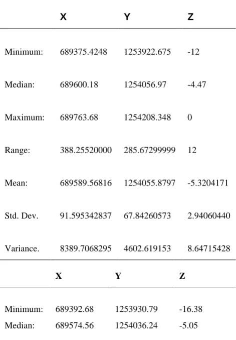
[image:2.595.311.547.422.761.2]The total sample collected during2003 survey is 9569 samples and 2013 survey had samples. The statistics given below:
Table 1: Statistics of Survey data samples
X
Y
Z
Minimum: 689375.4248 1253922.675 -12
Median: 689600.18 1254056.97 -4.47
Maximum: 689763.68 1254208.348 0
Range: 388.25520000 285.67299999 12
Mean: 689589.56816 1254055.8797 -5.3204171
Std. Dev. 91.595342837 67.84260573 2.94060440
Variance. 8389.7068295 4602.619153 8.64715428
X Y Z
Minimum: 689392.68 1253930.79 -16.38
Maximum: 689686.35 1254137.86 -1.67
Range: 293.669999 207.070000 14.71
Mean: 689566.757 1254035.2029 -6.02597991
Std. Dev. 64.5687860 50.203359868 3.058804652
Variance. 4169.12813 2520.37734 9.356285903
2.2
Interpolation
Interpolation is a popular option in obtaining unknown and missing values from a known data set. Interpolation techniques are based on the principles of spatial autocorrelation, which assumes that closer points are more similar compared to farther ones (Arun, 2013).
2.2.1
Cubic spline method
The Clough–Tocher interpolation method, is based on a triangulation of the given set of scattered points. It uses a cubicinterpolation scheme within each triangle using bivariate cubic polynomials (Amidror, 2002). The Spline interpolation approach uses mathematical function to minimize the surface curvature, and also produce a smooth surface that exactly fits the input points (Arun, 2013). In order to create a piecewise C1 - continuous interpolation surface, the Clough–Tocher method requires the value and the gradient i.e. two partial derivatives at each of the three vertices for each triangle, and the normal derivative at the midpoint of each of the three edges to ensure that the normal slope matches across triangle boundaries. It is achieved by splitting each triangle of the original triangulation into three mini trianglesby joining each of the three vertices to the centroid and defining a bivariate cubic polynomial on each of the three mini triangles. This construction gives more degrees of freedom for satisfying the constraints. The key idea behind the Clough–Tocher method is to split each cubic polynomial patch into three cubic polynomial sub patches, in order to satisfy the C1 -continuity constraints with neighbor.
2.2.2
Triangulation with linear interpolation
This algorithm creates triangles by drawing lines between data points. The scattered points (𝑥𝑖, 𝑦𝑖) are located in the 𝑥, 𝑦plane; their values can be visualized as altitudes
𝑧𝑖over this plane. Therefore, the triangulation of the scattered points in the 𝑥, 𝑦plane induces a piecewise triangular surface over the plane, whose nodes are the points (𝑥𝑖, 𝑦𝑖 , 𝑧𝑖). The original points are connected in such a way that no triangle edges are intersected by other triangles. The result is a patchwork of triangular faces over the extent of the grid. This is a continuous surface made up of flat triangular pieces that are joined along edges which is an obvious generalization of broken line functions in one dimension. Each triangle defines a plane over the grid nodes lying within the triangle, with the tilt and elevation of the triangle determined by the three original data points defining the triangle. All grid nodes within a given triangle are defined by the triangular surface. Because the original data are used to define the triangles, the data are honored very closely. Triangulation with Linear Interpolation works best when your data are evenly distributed over the grid area. Data sets containing sparse areas result in distinct triangular facets on the map.
2.2.3
Nearest neighbor interpolation
The nearest neighbour interpolation technique assigns the value of the points whose centre is closest to the centre of the output cell. It is the interpolation technique for discrete, or categorical, raster data, such as surface mesh, because it does not change the value of the input cells. In this method the output value on the mesh point is the value of the nearest
neighbour to that mesh point cells (Yang, Kao, Lee, & Hung, 2004).
The simplest interpolation from a computational standpoint is the nearest neighbour, where each interpolated output point is assigned the value of the nearest sample point in the input mesh. The interpolation kernel for the nearest neighbour
Algorithm is defined as
ℎ(𝑥) = 1,0 ≤ |𝑥| ≤ 0.5 Eq. 6(a)
ℎ(𝑥) = 0,0.5 ≤ |𝑥| ≤ 1 Eq. 6(b)
2.2.4
Natural neighborhood interpolation
Natural neighbour is a weighted-average interpolation method. It creates a Delaunay Triangulation of input points and selects the closest node that form a convex hull around the interpolation point (Yang, Kao, Lee, & Hung, 2004).When the data points are distributed unevenly, this is the most appropriate interpolation methods. It has an advantage that we do not have to specify the radius, number of neighbours or weights. This method allows to create most accurate surfaces from dataset that are distributed sparsely or very linear in spatial distribution.
As the gridded data has average nose about 20-30 percent popular denoising filters which are not commercially usedthe standard software are tested and performance was evaluated.
2.3
Denoising Methodology
2.3.1
Savitzky-Golay
Savitzky and Golay proposed a method of data smoothing based on local least-squares polynomial approximation (Savitzky & Golay, 1964).This approach showed fitting a polynomial to a set of input samples and then evaluating the resulting polynomial at a single point within the approximation interval, equivalent to discrete convolution with a fixed impulse response. Although the frequency response of the unweighted Savitzky–Golay filter is poor in terms of straight-forward frequency separation , the interpretation of the output as the ‘automatic’ realization of a polynomial least-squares fitting procedure has made the SG filter a popular choice in spectroscopy , voltammetry, and other fields such as biomedical monitoring (Acharya, Rani, Agarwal, & Singh, 2016). Polynomial smoothing is the process which replaces the noisy samples by the values that lie on the smooth polynomial curves drawn between the noisy samples. For every polynomial order, the coefficients must be determined optimally such that the corresponding polynomial curve best fits the given data (Acharya, Rani, Agarwal, & Singh, 2016).
Instead of averaging the neighbouring data points, it creates a least square fit with a polynomial of high order over an odd sized window centred at the point. Another suitable approach of filtering is Wavelet domain transform. However, it depends on large filter parameters like wavelet type, thresholding policy, threshold estimation and decomposition level, etc.[16]. Compared to wavelet, S-Golay technique requires only two parameters which is to be set, i.e. the degree of the polynomial and the width of the window, and also effective since the smoothened signal and the derivatives can be calculated in a single step (Schafer, 2011).
International Journal of Computer Applications (0975 – 8887) Volume 180 – No.33, April 2018
𝑁 = 2𝑀 + 1And 𝑁 ≥ 𝑑 + 1, where 𝑑 is order of
polynomial. (Balan, Khaparde, Tank, Rade, & Takalkar, 2014)
If x is noisy signal with noisy samples 𝑥𝑛,
𝑛 = 0,1, . . . , 𝐿 − 1 and noise is reduced to obtain a smoothed output version 𝑦 which contains 𝑦𝑛,
𝑛 = 0,1, . . . , 𝐿 − 1, then input vector has
n =L input points and x = [x0, x1… xL-1] T
is replaced by N dimensional, having M points on each side of x.
𝑥 = [𝑥−,𝑀, … . , 𝑥−1, 𝑥0, 𝑥1, … , 𝑥𝑀]𝑇 Eq. 7(a)
The Smoothed output y is calculated as
𝑦 = 𝐵𝑥; Eq. 7(b)
The Savitzky-Golay filter coefficients b0, b1 …..are the
elements of matrix B.
𝐵 = [𝑏−,𝑀, … . , 𝑏−1, 𝑏0, 𝑏1, … , 𝑏𝑀]; Eq. 7(c)
𝐵 = 𝐺𝑆𝑇 Eq. 7(d)
𝑊ℎ𝑒𝑟𝑒 𝐺 = 𝑆 𝑆𝑆 , 𝑆 = 𝑠0, 𝑠1, … , 𝑠𝑑
𝑠0 𝑚 = 1; 𝑠1 𝑚 = 𝑚; 𝑠2 𝑚 = 𝑚2 𝑤ℎ𝑒𝑟𝑒 – 𝑑 ≤ 𝑚 ≤ 𝑑
The main advantage of the S-Golay filter is its ability to preservethe signal compared to other methods of filtering (Schafer, 2011). The performance of SGolay filter is much superior to the conventional filters, considered correct order and frame size is chosen. Adaptive SGolay filtering helps to select the optimal frame size and order considering that the impulse response of an S-G filter can be computed as samples of the 𝑁𝑡ℎdegree polynomial fit to the unit impulse sequence. Filter coefficients need to be evaluated just once for a given application which makes the filtering process simple, easy and fast. There are some important constraints in the use of polynomial fitting in general.
2.3.2
Adaptive Wiener filter
The Wiener filter estimates the desired random process by linear time-invariant (LTI) filtering of an observed noisy process, assuming known stationary signal and noise spectra, and additive noise (Haykin, 2001).
Consider, signal corrupted by Gaussian noise modelled as
𝑦(𝑖, 𝑗) = 𝑥(𝑖, 𝑗) + 𝑛(𝑖, 𝑗) Eq. 8(a)
Where𝑦(𝑖, 𝑗) is the noise measurement, 𝑥(𝑖, 𝑗) is the additive noise free mesh and 𝑛(𝑖, 𝑗) is the additive Gaussian noise.
The goal here is to remove noise or de-noise 𝑦(𝑖, 𝑗) and to obtain linear estimate 𝑥 (𝑖, 𝑗) which minimize the mean square error.
𝑀𝑆𝐸(𝑥 ) = 1
𝑁 𝑥 𝑖, 𝑗 − 𝑥 𝑖, 𝑗
2 𝑁
𝑖,𝑗 =1 Eq. 8(b) Where N is the number of elements in 𝑥(𝑖, 𝑗)
When 𝑥(𝑖, 𝑗) and 𝑥 (𝑖, 𝑗) are stationary Gaussian process
And,
𝑥 (𝑖, 𝑗) = 𝜎𝑥2(𝑖,𝑗 )
𝜎𝑥2 𝑖,𝑗 +𝜎𝑛2(𝑖,𝑗 ) 𝑦 𝑖, 𝑗 − 𝜇𝑥(𝑖, 𝑗) +𝜇𝑥(𝑖, 𝑗)Eq. 8(c)
Where𝜎2, 𝜇 are the signal variances and mean respectively, and where we will normally assume the mean of noise to be zero.
The local mean and local variance are calculated over a uniform moving average window.
𝜇 𝑥(𝑖, 𝑗) =
1
2𝑟 + 1 2 𝑦 𝑝, 𝑞 − 𝜇 𝑥(𝑖, 𝑗) 2−
𝑗 +𝑟 𝑞=𝑗 −𝑟 𝑖+𝑟 𝑝=𝑖−𝑟
𝜎𝑛2 Eq. 8(d)
But, it tends to disturb the mean and increase the variance near the edges. Thus the resulting de-noised image is poor. So, using weighted form of variance to estimate 𝜎𝑛2(𝑖, 𝑗) while still using the estimate of 𝜇𝑥(𝑖, 𝑗)
𝜎 𝑥2(𝑖, 𝑗) = 𝑤(𝑖, 𝑗, 𝑝, 𝑞) 𝑦 𝑝, 𝑞 − 𝜇 𝑥(𝑖, 𝑗) 2
𝑗 +𝑟 𝑞=𝑗 −𝑟 𝑖+𝑟 𝑝=𝑖−𝑟
Eq. 9(a)
To determine the non-stationary weight 𝑤(𝑖, 𝑗, 𝑝, 𝑞), the method suggested is using a monotonically decreasing function to put more confidence on the centre variance estimate. Rather than deterministic Gaussian weight which may contain abrupt edges and other changes in behaviour, it is far more appropriate to consider an adaptive approach to selecting 𝑤().
𝑤 𝑖, 𝑗, 𝑝, 𝑞 = 𝑘(𝑖, 𝑗)
1 + 𝑎 max[∈2, 𝑦 𝑖, 𝑗 − 𝑦(𝑝, 𝑞)2] Eq. 9(b)
Where we assert that 𝑤(𝑖, 𝑗, 𝑝, 𝑞) = 0 and 𝑘(𝑖, 𝑗) is a normalization constant given by
𝐾(𝑖, 𝑗) = 1
1+𝑎 max [∈2,𝑦 𝑖,𝑗 −𝑦(𝑝,𝑞)2]
−1
Eq. 9(c)
The quantities 𝑎 > 0 and ∈= 2.5𝜎𝑛are the parameters of the weight function, such that 𝑎 ∈2>>1 to exclude outliers from the weight function 𝑤().In the result,both the local mean and the local variance are estimated adaptively.
𝜇 𝑥(𝑖, 𝑗) = 𝑖+𝑟𝑝=𝑖−𝑟 𝑗 +𝑟𝑞=𝑗 −𝑟𝑤 𝑖, 𝑗, 𝑝, 𝑞 𝑦(𝑝, 𝑞) Eq. 9(d)
𝜎 𝑥2(𝑖, 𝑗) = 𝑤(𝑖, 𝑗, 𝑝, 𝑞) 𝑦 𝑝, 𝑞 − 𝜇 𝑥(𝑖, 𝑗) 2
𝑗 +𝑟 𝑞=𝑗 −𝑟 𝑖+𝑟 𝑝=𝑖−𝑟
Eq. 9(e)
2.3.3
Least Mean Square Filter
The simplicity and relatively fewer computational operations makes Least Mean Square (LMS) a favorable approach in approximation of unknown signal (Haykin, 2001). The LMS algorithm is based on method of steepest decent. In TDLMS, the next weight matrix is equal to the present weight matrix plus the change proportional to the negative gradient (Hadhoud & Thomas, 1988).
𝑊𝑗 +1= 𝑊𝑗− 𝜇𝐺𝑗 Eq. 10(a)
Where,𝑊𝑗 is the weight matrix before updating, 𝑊𝑗 +1 is the weight matrix after updating, 𝜇 is the Scalar multiplier controlling the rate of convergence and filter stability, 𝐺𝑗 is the estimate for the 2-D instantaneous gradient of 𝐸[𝑒𝑗2] w.r.t.
𝑊𝑗. 𝐺𝑗 = 𝜕𝐸 [𝑒𝑗2]
𝜕𝑊𝑗 Eq. 10(b)
International Journal of Computer Applications (0975 – 8887) Volume 180 – No.33, April 2018
𝐺𝐼 𝑙, 𝒌 = 𝑑 𝑒𝑗2
𝑑𝑊 𝑊 = 𝑊𝑗 𝐼, 𝑘
= 2𝑒𝑗{ 𝜕𝑒𝑗
𝜕𝑊} 𝑊 = 𝑊𝑗(𝐼, 𝑘) Eq. 11(a)
The error signal 𝑒𝑗at the jthiteration is then defined as
𝑒𝑗 = 𝐷 ( 𝑚 , 𝑛 ) − 𝑊𝑗( 𝑙 , 𝑘 ) 𝑋 ( 𝑚 − 𝑙 , 𝑛 − 𝑘 )
𝑁−1 𝑘=0 𝑁−1 𝑙=0
Eq. 11(b)
From above equations Eq. 6(a) and Eq. 6(b),
{𝜕 𝑒𝑗
𝜕𝑊} 𝑊 = 𝑊𝑗 𝐼, 𝑘 = −𝑋(𝑚 − 𝑙, 𝑛 − 𝑘) Eq. 12
Then,
𝐺 (𝑙 , 𝑘) = − 𝑋 ( 𝑚 − 𝑙 , 𝑛 − 𝑘 ) Eq. 13(a)
Or the estimated instantaneous gradient matrix GI is
𝐺 𝐼 = − 𝑥𝑧 Eq. 13(b)
Substituting, we get
𝑊𝑗 +1= 𝑊𝑗 + 2𝜇. 𝑒𝑗. 𝑥𝑗 , which can be rewritten as
𝑊𝑗 +1(𝑙, 𝑘) = 𝑊𝑗(𝑙, 𝑘) + 2𝜇. 𝑒𝑗. 𝑋 ( 𝑚 − 𝑙 , 𝑛 − 𝑘 ) Eq. 14
3.
RESULTS AND DISCUSSION
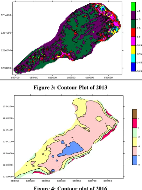
[image:5.595.50.279.69.356.2]Three different survey data over different time period i.e. 2003, 2013 and 2016 are considered (shown in Figure 1, Figure 2 and Figure 3) of the same lake is considered for evaluating for the algorithm, which is developed to improve the SNR and get minimum mean square error. The 2016 bathymetry data (Figure 3) was used as the reference since during that survey most of the underwater vegetation and sediments were dredged out. During this measurements the water level was at minimum and hence most of the elevation were collected with RTK system and was accurate up to few mm. Hence it was appropriate for the comparison of the results obtained with the calculated volume.
[image:5.595.316.543.74.377.2]Figure 2: Contour Plot of 2003
Figure 3: Contour Plot of 2013
Figure 4: Contour plot of 2016
All the mentioned interpolation methods are used to grid the data and a common region of interest, of size 167m x 150m, by applying a boundary extracted from the GPS coordinates.
In the Pre-filtering, the statistical analysis is done. The variance of both northing and easting distance are analyzed (shown in Figure 4). The variance shows the distribution of the noise present in the data which is vital for analyzing the region of interest.
The Denoising performance of the filter is done by Mean Square Error (MSE), Peak Signal to Noise ratio (PSNR) and correlation.The test conducted on an I3 core CPU with each processor running at 3.2 GHz clock speed and 4GB of RAM. The program was run and compiled in MATLAB.
To estimate the performance quality, Mean Squared Error are calculated for the original and the Filtered data. Performances are tested by calculating MSE and PSNR. The values are calculated by the following expressions:
𝑀𝑆𝐸 = 1
𝐿 𝑋 𝑖 − 𝑌 𝑖
2 𝐿−1
𝑖=0 Eq. (15)
PSNR = 10log10
𝐿2
𝑀𝑆𝐸 Eq. (16)
Where𝑋 𝑖 is the noise-free original data, 𝑌(𝑖) is the predicted filtered data and𝐿 is the length of the data.
𝐶𝑂𝑅 = 𝑛𝑖=1(𝑥𝑖−𝑥 )(𝑦𝑖−𝑦 )
𝑛𝑖=1((𝑥𝑖−𝑥 ))2 𝑛𝑖=1(𝑦𝑖−𝑦 )2
Eq. (17) 689400 689450 689500 689550 689600 689650 1253950
1254000 1254050
-3 -2.6 -2.2 -1.8
689400 689450 689500 689550 689600 689650 1253950
1254000 1254050 1254100
-16.5 -14.5 -12.5 -10.5 -8.5 -6.5 -4.5 -2.5
689450 689500 689550 689600 689650 689700 689750 1253950
1254000 1254050 1254100 1254150 1254200 1254250
[image:5.595.56.280.485.631.2]International Journal of Computer Applications (0975 – 8887) Volume 180 – No.33, April 2018
Figure 5: Variance plot along the Easting and Northing
The MSE, PSNR and Correlation for 2003 and 2013 data are shown in Table 1;
Table 2: MSE, PSNR and Correlation forAdaptive Filters(2003 and 2013)
Adaptive
Filter
2003 2013
MSE PSNR (dB)
COR MSE PSNR (dB)
COR
Wiener 2.202 40.559 0.845 2.847 39.444 0.7848
LMS 2.346 40.283 0.808 2.978 39.247 0.746
[image:6.595.53.544.81.760.2]Analysis for Savitzky-Golay filter is done for different order and frame size. And the performance is showed in table 2 and 3.
Table 3: MSE, PSNR, Correlation comparison at different orders and frame size of SGolay Filter. (Year 2003)
Order
of
polynomial
Frame
Size
MSE
PSNR
COR
1
15
1.869
41.270
0.802
31
0.593
46.255
0.701
41
0.386
48.119
0.6320
3
15
2.215
40.533
0.782
31
0.981
44.067
0.683
41
0.665
45.758
0.620
5
15
2.370
40.239
0.776
31
1.184
43.252
0.675
41
0.833
44.778
0.613
7
15
2.473
40.054
0.773
31
1.292
42.876
0.670
41
0.942
44.247
0.608
Table 4: MSE, PSNR, Correlation comparison at different orders and framesize of SGolay Filter (Year 2013)
Order
of
polynomial
Frame
Size
MSE
PSNR
COR
1
15
1.869
41.270
0.7326
31
1.284
42.90
0.6302
41
0.865
44.614
0.5701
3
15
2.215
40.533
0.7192
31
1.025
43.87
0.6176
41
0.662
45.774
0.5584
5
15
2.370
40.239
0.7135
31
1.356
42.663
0.6147
41
0.894
44.469
0.5568
7
15
2.473
40.054
0.7098
31
1.435
42.418
0.6118
41
0.944
44.235
0.5546
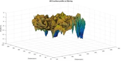
Figure 6: Original Surface Plot 2003
[image:6.595.281.538.86.721.2]Figure 7: Filtered Surface Plot 2003
[image:6.595.49.283.486.765.2]Figure 9: Filtered Surface Plot 2013
Among the adaptive filters, wiener filter had better performance compared to LMS both in terms of PSNR and correlation with at least 10% better SNR in both the cases. On comparison of S-Golay with the orders and frame size,
In case of S-Golay filter analysis, for 2003 data analysis, SG Filter of 1st order and frame size of 31 and, in case of 2013 data analysis, 3rd order S-Golay filter with frame size 31 had better performance, by also considering degradation in correlation with the increasing frame size.
4.
CONCLUSION
The data analysed in this paper is collected from an Indian reservoir which suffers huge sedimentation due to the terrain conditions as well as the vegetation practices followed in this region. There are no guidelines to suggest the data analyst to select the algorithm based on the site condition and hence filtering and interpolation are left to the analyst to decide and hence sediment volume could not be assessed precisely. All the technologies and calculations done with existing commercial software are developed for different site conditions across the world, which does not always suite Indian conditions, ends up estimating the capacity with considerable error. The data used in this paper covers a period of ten years and the technology changed during the course of time. However the processing techniques was the same and hence it was required by us to develop customized algorithms in the data processing. The adaptive filters and S-Golay filters are designed and applied for acoustic bathymetry data based on the signal conditions. The design parameters of the filter are varied in a certain feasible range and all the possible combinations are evaluated using a systematic procedure. The filters were applied to data obtained at two different period of 2003 and 2013. The PSNR and MSE value depicts better value of with the increase in frame size. However, there is a considerable degradation in correlation at the same time indicating the data is becoming more uncorrelated with the increasing frame size. Therefore, for 2003 data analysis, SG Filter of 1st order and frame size of 31 is preferred. While, in case of 2013 data analysis, 3rd order S-Golay filter with frame size 31 is selected. Among the adaptive filters, Adaptive wiener had a better performance than LMS filter. The results were improved in terms of sediment volume calculations, which got validated against the dredging volume. Hence this study recommends use of site specific filter, interpolation and signal processing methods and not to use the generalized tools.
5.
ACKNOWLEDGMENTS
The authors sincerely acknowledge, Dr. Surendra Pal, Vice Chancellor of DIAT (DU) Pune, Director of CWPRS Pune for motivation, the Garrison Engineers, Wellington and the team of officials for providing necessary support during data collection. The authors are also grateful to| Mr. Raghak Radhakrishnan, Trainee student, CWPRS who helped in the editing this paper.
6.
REFERENCES
[1] Acharya, D., Rani, A., Agarwal, S., & Singh, V. (2016). Application of adaptive Savitzky-Golay filter for EEG signal processing. Elsevier Perspectives in Science , 677—679.
[2] Agarwal, S., Rani, A., Singh, V., & Mittal, A. P. (2015). Performance Evaluation and Implementation of FPGA Based SGSF in Smart Diagnostic Applications. Journal of Medical Systems , 40 (3), 63.
[3] Amidror, I. (2002). Scattered data interpolation methods for electronic imaging systems: a survey. Journal of Electronic Imaging , 11 (2), 157-176. [4] Arun, P. (2013). A comparative analysis of different
DEM interpolation methods. The Egyptian Journal of Remote Sensing and Space Sciences , 133–139. [5] Balan, S., Khaparde, A., Tank, V., Rade, T., &
Takalkar, K. (2014). Under water noise reduction using wavelet and savitzky-golay. (pp. 243–250). Second International Conference on Computational Science and Engineering.
[6] Fernandes, Chakraborty, B., & William. (2012). Bathymetric Techniques and Indian Ocean Applications. Intech:Europe , 1-29.
[7] Hadhoud, M. M., & Thomas, D. W. (1988). The two-dimensional adaptive LMS (TDLMS) algorithm. IEEE Transactions on Circuits and Systems , 35 (5), 485-494. [8] Haykin, S. (2001). Adaptive Filter Theory (3 ed.).
Prentice Hall.
[9] Jarrot, A., Ioana, C., & Quinquis, A. (2005). Denoising underwater signals propagating through multi-path channels. In Europe Oceans (pp. 501--506). IEEE.
[10]Mohammed, N. Z., Ghazi, A., & Mustafa, H. E. (2013). Positional accuracy testing of Google Earth.
International Journal of Multidisciplinary Sciences and Engineering , 4 (6), 6-9.
[11]Sadaf, S., Yashaswini, P., Halagur, S., Khan, F., & Rangaswamy, S. (2015). A Literature Survey on Ambient Noise Analysis For underwater Acoustic Signals. International Journal of Computer Engineering and Sciences , 1 (7).
[12]Savitzky, A., & Golay, M. J. (1964). Smoothing and differentiation of data by simplified least squares procedures. Analytical chemistry , 36 (8), 1627-1639.
International Journal of Computer Applications (0975 – 8887) Volume 180 – No.33, April 2018
35 [14]Selva Balan. (2016). Hydrological Survey of Lower
Lake at Kateri belongs to Cordite Factory, Aruvankadu, using Single Beam Echo Sounder, Real Time Kinematic (RTK) DGPS technique, and Total Station. No:5399. Department of Hydrolic Instrumentation. PUNE: CWPRS.