Deep verification learning

University of Twente

Department of Services, Cybersecurity and Safety

Master Thesis

Deep Verification Learning

Author:

F.H.J.

Hillerstr¨

om

Committee:

Prof. Dr. Ir. R.N.J.

Veldhuis

Dr. Ir. L.J.

_Spreeuwers

Dr. Ir. D.

_Hiemstra

Deep Verification Learning

Fieke Hillerstr¨

om

December 5, 2016

Abstract

Deep learning for biometrics has increasingly gained attention over the last years. Due to the expansion of computational power and the increasing sizes of the available datasets, the performance has surpassed that of humans on certain verification tasks. However, large datasets are not available for every application. Therefore we introduce Deep Verification Learning, to reduce network complexity and train with more modest hardware on smaller datasets. Deep Verification Learning takes two images to be verified at the input of a deep learning network, and trains directly towards a verification score. This topology enables the network to learn differences and similarities in the first layer, and to involve verification signals during training. Directly training towards a verification score reduces the number of trainable parameters significantly. We applied Deep Verification Learning on the face verification task, also it could be extended to other biometric modalities. We compared our face verification learning topology with a network trained for multi-class classification on the FRGC dataset, which contains only 568 subjects. Deep Verification Learning performs substantially better.

1

Introduction

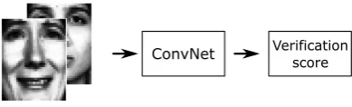
Deep learning face recognition has been extensively studied during the last years and has obtained impressive results [2–6]. Deep learning methods automatically learn to extract the discriminative features for the task they are trained on. The increasing availability of computational power and training data allows dor the training of deeper networks, and has increased the recognition performances immensely. We introduce Deep Verification Learning to reduce the network complexity and enable training on smaller datasets (see Figure 1).

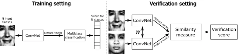
Most of the state-of-the-art deep learning face recognition systems use convolutional networks (abbreviated ConvNets). For face verification, commonly a framework based on multi-class classification is used [5] (see Figure 2). The classification layer of the network is removed, whereafter a feature vector remains. The network is replicated and on top of these feature vectors, a new verification layer is trained (see Figure 2). We define this type of learning as ‘Identification Learning’. The state-of-the-art systems are trained with the currently available large datasets and achieve excellent performances.

One of the challenges in deep learning face recognition is data bias [5]. The deep networks are usually trained with large datasets, but do not generalize well to new face verification

ConvNet Verification_score

Figure 1: Deep Verification Learning. Two images are presented as input of the network and the system is directly trained towards a verification score. Face images are preprocessed images from the FRGC dataset [1].

Training setting Verification setting

ConvNet

Similarity

measure Verification score

W Featur

e v ector

Featur e vector

ConvNet

ConvNet Feature vector _{classification}Multiclass

Score for N classes N input

classes

Figure 2: Identification Learning convolutional network. Left: Training for multi-class classification. Right: Two networks are replicated in verification setting. The networks have the same fixed weightsW. A new top-layer is trained. Face images are preprocessed images from the FRGC dataset [1].

Dataset #Images #Subjects Access Source

LFW [7] 13,233 5,749 Public Celebrity search

CelebFaces+ [8] 202,599 10,177 Public Celebrity search CASIA-WebFace [9] 494,414 10,575 Public Celebrity search MS-Celeb-1M [10] 10M 100K Public Celebrity search Social Face Classification

(Facebook) [2]

4.4M 4,030 Private Facebook

Google [4] 100-200M 8M Private Undefined

Megvii Face Classification [5] 5M 20K Private Celebrity search

FRGC [1] 39,328 568 Public Photo sessions

Table 1: Datasets used for training deep learning face recognition networks and their char-acteristics.

applications. Depending on the type of application, the availability and sizes of the datasets differ (see Table 1). The availability of training data is limited for applications that do not utilize public web images. For those applications, like access or border control, it is interesting to investigate less complex deep learning architectures, that train on smaller datasets.

We propose a Deep Verification Learning system, directly trained for a verification score, applied for face recognition (see Section 3). We applied Deep Verification Learning on the task of face recognition and it could be extended towards other biometric modalities. We hypothesize that Deep Verification Learning will outperform an Identification Learned network on the face verification task, when small datasets are used. Deep Verification Learning offers several advantages over Identification Learning. Training a network in pairs enables the creation of extra training samples. Providing two images as input of the network enables it to learn face similarities and differences directly at the first layers, and to use these in the higher layer. Training towards a verification score instead of multi-class classification reduces the number of network parameters drastically. In our experiments, for example, the number of parameters reduces from 36,316 for Identification Learning to 13,772 for Deep Verification Learning. Given these advantages, we hypothesize that our network can train more effectively on small datasets.

We investigate the ability of Deep Verification Learning by comparing Deep Verification Learning with Identification Learning (see Section 4). We explore the benefits of increasing the dataset size in a controlled manner. The research questions addressed in this paper are:

1. Can Deep Verification Learning result in similar or better face verification performance then Identification Learning?

(a) What is the effect of the number of images per subject in a dataset on face verification performance?

(b) What is the effect of the number of subjects in a dataset on face verification performance?

We will first describe the related background for our research in Section 2. We explain the details of Deep Verification Learning in Section 3, whereafter we describe our experiments. Finally we present our conclusions and recommendations.

2

Related Work

Face verification has gained the interest of researchers for several decades, improving its performance. Traditional face verification systems use model-based features (e.g. LBP [11] and Gabor wavelets [12]), often combined to enhance performance. Deep learning systems are able to automatically learn the important features from the input, which eliminates the need for model-based features.

Deep learning face verification systems typically incorporate the spatial information in images by using convolutional networks [2, 3,5,13]. Convolutional networks reduce the num-ber of parameters in a network, allowing for deeper topologies. Commonly, a framework based on multi-class classification is taken [5]. The networks are trained for a multi-class classification task, to identify all the subjects in the training set (see Figure 2). The iden-tification layer is removed and a feature vector remains. A similarity measure is added for verification (see Figure 2). We define this type of training as ‘Identification Learning’. Dif-ferent types of top layers can be used. Examples of untrained methods are the inner product between two normalized feature vectors [2] or the L2 norm [5]. Possible trained methods are the weighted-χ2 distance, Joint Bayesian [14], and a new-trained neural network [14]. Deep-Face [2] takes a Siamese network and trains a top softmax-layer, which takes the absolute difference between two feature vectors as input, to predict a similarity score. They report overfitting to the trainingdata when fine-tuning the Siamese pre-trained feature extractor. However, in an ensemble it enhanced the verification accuracy.

Most of the traditional and deep learning topologies extract the features of two faces separately. Verification signals can be incorporated in the learning process to enhance train-ing. DeepID2 [15] combines verification and identification signals into a joint cost function with a hyperparameterλ. The fully connected layer is connected to the last convolutional layer and the last max-pooling layer. FaceNet [4] uses a triplet loss function during training, which minimizes the distance between genuine pairs and maximizes the distance between imposter pairs, by using feature vectors of three images in the loss calculation. The triplets used for training are selected depending on the verification difficulty.

Typically the networks contain multiple convolutional layers in combination with max-pooling layers and followed by fully-connected layers. Because different face regions have different local statistics, locally connected layers could be used in the higher layers [2, 13, 14]. Locally shared weights enable the extraction of specific features from different face regions and was first introduced by Hung et al. [28]. An ensemble of multiple networks trained for different face regions could enhance performance [5, 14]. Most architectures use the output of a non-final fully-connected layer as feature vector for face verification. Deep Verification Learning trains directly towards a verification score, instead of using an intermediate representation.

The datasets used for training these deep networks are commonly large and contain mostly public available web images (see Table 1). The trained networks do not generalize well to new applications, as investigated by Zhou et al. [5]. They found a big gap in performance when transferring a convolutional network trained on a large dataset of celebrities from the internet, towards a real-world security application. In case of controlled applications, only small datasets are available. Deep Verification Learning trains in pairs, which enlarges the

Figure 3: System architecture of the hybrid ConvNet-RBM model, proposed by Sun et al.. Image from [13].

number of training batches. It reduces the number of parameters in the network as follows: with a dataset of N subjects, the last layer of an Identification Learning network is an

N-way softmax-layer. If the second last layer has a length K, the number of parameters for this last fully-connected softmax-layer isK·N. In case of Deep Verification Learning the output softmax-layer is a two-way softmax-layer, causing for 2·K parameters. Deep Verification Learning reduces the number of parameters to be trained significantly. Because of this considerable parameter reduction, we hypothesize that Deep Verification Learning outperforms Identification Learning.

Sun et al. [13] proposed a similar verification learning architecture, which takes two images at the input and is trained towards a verification score (see Figure 3). They train twelve groups, each containing five different convolutional networks. The twelve groups are trained for different face regions, some in color, some in gray values. The five networks in every group are trained on different bootstraps of training data. They average the output of eight different input modi (flipped and exchanged input region pairs). The outputs of those 5x12 convolutional networks are two times averaged pooled and followed by a top layer classification RBM. However, their architecture is rather complex and trained on a large dataset, CelebFaces, containing 87,628 images of 5,436 persons. Our aim is to design a less complex network that can train on smaller datasets. Therefore we propose a simplified version of the architecture proposed by Sun et al., containing a basis of their proposed network.

3

Deep Verification Learning

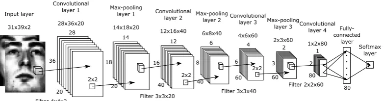
We introduce a Deep Verficication Learning network, based on the architecture proposed by Sun et al. [13]. The network takes two images as input and is directly trained towards a ver-ification score. The proposed topology is shown in Figure 4 and contains four convolutional layers, which enables it to extract features hierarchically. The first three convolutional layers are each followed by a max-pooling layer, which provides a simple rotation and translation invariance. The Rectified Linear Unit (ReLU)f(x) = max(0, x) [16] is used as activation function. Two grayscale images are presented as input of the network, each in a separate channel. The expected dimensions of the input images are 31x39 pixels (WxH). A fully-connected layer is fully-connected to the last convolutional layer, to be able to fuse the outputs of the different filters. The fully-connected layer is followed by a two-way softmax-layer;

pt = e

xi

. . . . 20 28 36 Convolutional layer 1 28x36x20 14 18 20 Max-pooling layer 1 14x18x20 2x2 Input layer 31x39x2

Filter 4x4x2 Filter 3x3x20 Convolutional layer 2 12x16x40 12 16 40 6 8 40 2x2 Max-pooling layer 2 6x8x40 4 6 60 Filter 3x3x40 Convolutional layer 3 4x6x60 2 3 60 2x2 Max-pooling layer 3 2x3x60 1 2 80 Filter 2x2x60 Convolutional layer 4 1x2x80 Fully-connected layer Softmax layer 80

Figure 4: Deep Verification Learning convolutional network. At the input two grayscale images are presented, each in a separate channel. The network is directly trained towards a verification score. Network based on the topology proposed by Sun et al. [13]. Face images are preprocessed images from the FRGC dataset [1].

predicts a chance for two classes, genuine pairs and imposters pairs. Because the outputs of the softmax add up to one, the score for the genuine class is used as verification score, with a score of one belonging to genuine pairs and zero to imposter pairs.

Hu et al. [17] evaluated the use of RGB and grayscale images for face recognition convo-lutional networks and found that colour images do not deliver a notable improvement. Using grayscale images reduces the complexity of the network and the number of parameters to be trained. To limit the number of parameters, only a single model is trained with the full facial area as input. We did not apply model averaging or models trained for specific facial regions. The number of parameters in the network, excluding the final softmax-layer, is 13,612. The softmax-layer adds 160 parameters. In the case of Indentification Learning, the final softmax-layer adds 80·N parameters, which increases the trainable parameters in the network immensely. With 170 subjects, the number of parameters would have doubled. As can be seen in Table 1, datasets used for training deep networks have way more subjects than 170 and Deep Verification Learning thus reduces the number of parameters significantly.

4

Experiments

We compared the Deep Verification Learning system to an Identification Learned convo-lutional network, to evaluate the advantages of our proposed training architecture. The networks are compared in three experiments, related to the research questions. The first experiment evaluates the verification performance of both Deep Verification Learning and Identification Learning. The second and third experiment explore the benefits of increasing the dataset-size in a controlled manner, in which a distinction is made between a dataset increase via extra subjects or via extra images per subject.

4.1

Experiment setup

4.1.1 Network architectures

The architectures of both systems to be compared are identical, except for the input and output layer. The Deep Verification Learning network is shown in Figure 4 and discussed in Section 3. The Identification Learned network is first trained for the classification task, as shown in Figure 5. The network is trained to output a probability score for the input to belong to one of theN classes, via anN-way softmax-layer. When training has completed, the classification layer is removed and a feature vector is obtained. The two feature vectors of the images to be compared are normalized to have zero mean and unit variance and taken as input for a new-trained two-way softmax-layer. WithxA andxB referring to normalized

feature vectors, the input for the softmax-layer is|xA−xB|(see Figure 6). Normalizing the

. . . . 80 . . . . N 20 28 36 Convolutional layer 1 28x36x20 14 18 20 Max-pooling layer 1 14x18x20 2x2 Input layer 31x39

Filter 4x4 Filter 3x3x20 Convolutional layer 2 12x16x40 12 16 40 6 8 40 2x2 Max-pooling layer 2 6x8x40 4 6 60 Filter 3x3x40 Convolutional layer 3 4x6x60 2 3 60 2x2 Max-pooling layer 3 2x3x60 1 2 80 Filter 2x2x60 Convolutional layer 4 1x2x80 Fully-connected layer Softmax layer

Figure 5: Training the convolutional network for multi-class classification. Single images are provided at the input, belonging to N subjects. The N-way softmax-layer calculates a probability score for theseN subject classes. Face images are preprocessed images from the FRGC dataset [1].

80 |A - B|

Softmax layer

Same fixed weights

Additionally trained . . . . 80 20 28 36 14 18 20 2x2

Filter 4x4 Filter 3x3x20 12 16 40 6 8 40 2x2 4 6 60 Filter 3x3x40 2 3 60 2x2 1 2 80 Filter 2x2x60 Feature Vector A . . . . 80 20 28 36 14 18 20 2x2

Filter 4x4 Filter 3x3x20 12 16 40 6 8 40 2x2 4 6 60 Filter 3x3x40 2 3 60 2x2 1 2 80 Filter 2x2x60 Feature Vector B

Figure 6: Identification Learned convolutional network for face verification. The networks are trained on multi-class classification (see Figure 5) and are identical. The feature vec-tors of both images are taken as input for a two-way softmax-top-layer. Face images are preprocessed images from the FRGC dataset [1].

input vectors turned out to result in higher verification performances in our experiments, probably because the ReLU activation function is activated at zero and expects the input data to be zero centered. Similar to Deep Verification Learning, one of the two outputs is taken as verification score. The weights of the networks are shared and fixed when training the new softmax-layer.

4.1.2 Training settings

The networks are trained using mini-batch stochastic gradient descent with backpropagation and a mini-batch size of 32. Before every epoch, the order of the training samples is shuffled. The learning rate is fixed at 0.005. These training settings are based on recommendations by Bengio in [18]. The cost function is the negative log-likelihoodC(x) = −log(pt), with

t denoting the target class. The cost function is normalized to the number of samples in target classt, to compensate for an unbalanced dataset. Xavier initialization [19] is used to initialize the weights and the biases are initialized to zero.

Learning validation set contains single face images from theN target classes in the training set. During a training epoch, the cost on the validation set is evaluated after training every ten mini-batches. The parameters resulting in the lowest cost on the validation set are saved as ‘best parameters’. When training does not improve the cost on the validation set for sev-eral epochs, training is stopped and the saved ‘best parameters’ are taken as final model. When training for multi-class classification, the rank-1 recognition score of the Identifica-tion Learning validaIdentifica-tion set is evaluated after every epoch. Because the validaIdentifica-tion set for multi-class classification contains images of the same subjects, overfitting on these subjects can occur. To reduce this effect, the ‘best parameters’ are only updated if these parameters result in the lowest rank-1 recognition score. When this rank-1 recognition score does not improve for several epochs, training is stopped and these ‘best parameters’ are taken as the parameters of the final model.

4.1.3 Datasets & preprocessing

The first experiment is performed using the controlled images of the FRGC dataset [1], which contains 24,614 controlled images, from 568 subjects. The second and third experiment use a combination of twelve different public datasets, merged and used by Zeng et al [21]. These combined datasets contain 438,319 images of 13,671 subjects. For both datasets, 50% of the subjects is used for the training set, the other 50% for the validation set which is used for the final model evaluation and in the early stopping algorithm. Using the validation set for both the model evaluation and in the early stopping algorithm adds a bias to the results. The bias occurs in the decision when the networks start to overfit on the training set and when training should be stopped. The validation set is not used for updating the parameters itself. Therefore the images in the validation set do not influence the features that are learned. For a particular training set and network combination we expect that the network starts overfitting around the same number of training iterations when tests are repeated. All models in the comparison are trained and evaluated using the same method and same validation set and thus contain the same bias. Looking at these arguments we expect the bias in the results to be small and to have no influence on the comparison.

The input images are preprocessed, before presenting them to the network. They are converted to grayscale values and registered on the eyes, using annotated coordinates. The images are cropped to a fixed box around the eyes’ coordinates and scaled to a fixed size of 31x39 pixels. Thereafter the images are histogram equalized and converted to have zero mean, in order to provide a balanced input for the ReLU. When training the convolutional network for multi-class classification, the network is trained on single images and their target subject class. From all the available images in a training set 90% is randomly selected for actual training, the remaining 10% is used for validation in the early stopping algorithm. Deep Verification Learning trains with genuine and imposter pairs, equal in number. The number of genuine pairs Ngen that could be generated, increases quadratically with the

number of imagesNim per subjectNgen =Nim·(Nim−1)· 1₂. To keep the training data

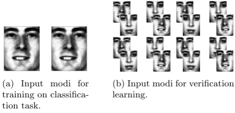
balanced, a maximum is set on the number of genuine pairs generated per subject, specified for each test later on. Data augmentation is applied in the training set, by adding all possible modi (see Figure 7). In the validation sets, the genuine and imposter pairs are equally distributed over the subjects.

4.2

Performance comparison

The first research question is studied by comparing the two architectures on their verification performance. The performances are evaluated using the controlled images of the FRGC dataset. The subjects are randomly split in training and validation sets. The details of the sets are specified in Table 2. The Deep Verification Learning dataset contains genuine pairs for every subject, with a maximum of 66 pairs. In the validation set the genuine pairs are equally distributed. The initialization and training of both networks is repeated five times

(a) Input modi for training on classifica-tion task.

(b) Input modi for verification learning.

Figure 7: Data augmentation is used for the training set.

#Subjects #Images #Training pairs Training set verification 284 11,920 32,136 Validation set identification 284 1,192 -Validation set verification 284 12,694 10,000

Table 2: Dataset details for the performance comparison.

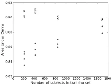
with the exact same dataset, to diminish the variations. The ROC curves of all ten tests are shown in Figure 8. The ROC curves of the Identification Learning networks show a higher variance than in Deep Verification Learning. The variance in the Area Under Curve (AUC) is 1.4×10−6 _{and 3.0×10}−8_{, respectively. We selected one of the networks trained}

for multi-class classification and re-training the top layer five times, to explore the cause of this variance. The ROC curves of these retrained top layers are shown in Figure 9 and the variance in the AUC is 3.0×10−9_{. We conclude that the variance in performance is created}

in the first training stage, when the network is trained for the multi-class classification task. The verification performance of an Identification Learned convolutional network is highly dependent on the multi-class classification training. We expect that the difference in variance is caused by the high number of trainable parameters. The Deep Verification Learning model has only 13,772 parameters to train, as opposed to the 36,316 parameters of the Identification Learning network. With a dataset of only 10,728 training images, it is likely that the multi-class classification network overfits and depends more heavily on the randomness of initialization and training.

Deep Verification Learning performs substantially better than Identification Learning in our experiments. However, some remarks have to be made. Only one type of newly-trained top layer for Identification Learning is evaluated. Other types of top layers could enhance the verification performance. The dataset used for testing has its limitations. Only the controlled images are used, which limits the diversity in images. The number of images is low compared to the number of parameters in the networks, especially in the case of Identification Learning this can lead to overfitting. Further experiments should be done on datasets with a higher variety. In our experiments we limited the number of genuine pairs per subject, to keep the dataset balanced. More training pairs could be formed and may increase the verification performance when all possible genuine pairs are used in a balanced way. In that case certain genuine pairs could be presented more frequently during training, or the cost function could be normalized towards the subject occurrence in the dataset.

4.3

Dataset configuration comparison

Figure 8: ROC curves for the five Deep Ver-ification Learned networks (black) and the five Identification Learned networks (gray) on the FRGC controlled dataset.

Figure 9: ROC curves for the five re-trained top layers with the same fixed convolutional network.

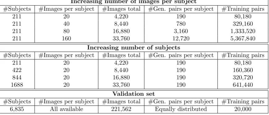
Increasing number of images per subject

#Subjects #Images per subject #Images total #Gen. pairs per subject #Training pairs

211 20 4,220 190 80,180

211 40 8,440 780 329,160

211 80 16,880 3,160 1,333,520

211 160 33,760 12,720 5,367,840

Increasing number of subjects

#Subjects #Images per subject #Images total #Gen. pairs per subject #Training pairs

211 20 4,220 190 80,180

422 20 8,440 190 160,360

844 20 16,880 190 320,720

1688 20 33,760 190 641,440

Validation set

#Subjects #Images per subject #Images total #Gen. pairs per subject #Training pairs 6,835 All available 221,562 Equally distributed 20,000

Table 3: Dataset details for testing with increasing number of images per subject, increasing number of subjects in the dataset, and the validation set.

the number of images per subject and subjects in a dataset in a comparable manner. The composition of the datasets in both tests are summarized in Table 3. 50% Of the subjects are used in the training set, from which the training data for every test is sampled. The validation set is kept the same in every test. Because the numbers of images per subject is equal over the whole dataset, every possible genuine pair is generated. The networks are trained on the datasets specified in Table 3 and tests are repeated three times.

The Area Under Curve values of these tests are shown in Figures 10 & 11. Adding extra images per subject to the dataset gives remarkable results. Contrary to the expected increase in performance, the performance in fact declines. The Deep Verification Learning performance is more affected by this than Identification Learning is. We expect that the decline in performance is caused by the network strongly overfitting on the training data. Because only the subjects with 160 images or more are used in the training set and the training data is sampled from a set of combined datasets, there is a bias in the datasets used for the training data. It turned out subjects from only two datasets, Multi-PIE [22] and CASIA-WebFace [23], met this requirement of containing a minimum of 160 images per

Figure 10: Area Under Curve values for the Deep Verification Learned networks (x) and the Identification Learned networks (o), for different number of images per subjects in the dataset.

Figure 11: Area Under Curve values for the Deep Verification Learned networks (x) and the Identification Learned networks (o), for different number of subjects in the dataset.

Test Imp. different datasets Imp. same datasets

80 Images per subject 0.729 0.469 0.693 0.719 0.735 160 Images per subject 0.542 0.514 0.684 0.718

844 subjects 0.899 0.898 0.902 0.898 0.900

1688 subjects 0.897 0.899 0.897 0.904

Table 4: AUC values for Deep Verification Learning network for different imposter pair construction in the trainingset. Imposters are formed within all the possible datasets (left) or imposter pair forming is restricted to subjects within the same dataset (right).

subject and were sampled into the training set. Creating these immense numbers of training pairs for only two type of datasets, causes overfitting to these types of data and prevents the networks from generalizing well on the new type of data from the validation set. We recommend repeating these experiments on datasets with the same type of images as those in the final application, to prevent creating a bias by overfitting on specific datasets.

Another remarkable result is found when increasing the number of subjects in the training set. For Identification Learning the performance increases, as expected. For Deep Verifi-cation Learning the performance declines when too many subjects are added. In this test, subjects in the training set are sampled from all subjects having 20 images or more. There-fore in this experiment more datasets are represented in the training set. A possible cause of the decline in performance could be the way the network learns. In case of Deep Verification Learning it is possible to learn to compare type of images (different datasets), instead of recognizing faces. When training in pairs, it is possible to compare the type of images for a genuine/imposter decision; different type of images are unlikely to form a genuine pair. When increasing the number of training pairs, this could cause overfitting to the type of images represented in the training set.

5

Conclusions & Recommendations

We introduced Deep Verification Learning and applied it to face verification. We compared Deep Verification Learning with networks trained for multi-class classification and evaluated the verification performance on the FRGC dataset, to answer our first research. Additionally we evaluated the effect of different dataset-sizes on the verification performance. We found a notable improvement in face verification performance when Deep Verification Learning is used instead of Identification Learning. Increasing the dataset-sizes does not improve the verification performances as expected, but in fact the performance declines. Care must be taken in training set selection, to prevent the networks from overfitting. Adding extra images or subjects from a type other than that used in the final application, creates a bias and counteracts the performance benefit from Deep Verification Learning.

Despite the promising results of our Deep Verification Learning network, more extensive experiments should be done. The experiments should be performed with a separate valida-tion set for the early stopping algorithm, which is not used in the final model evaluavalida-tion. This set should contain subjects that are not present in the training and test set. We recom-mend the use of cross-validation to better estimate the general verification performances of each network. The FRGC dataset is limited in variety and number of subjects. More uncon-trolled conditions and different types of datasets should be tested. The network should be compared to state-of-the-art face recognition systems, using one of the existing evaluation protocols. The tests regarding the influence of different dataset sizes, should be performed in a way that dataset bias is not possible. Ideally a large dataset with the same type of images is used, to avoid overfitting on one type of dataset.

The learning process is important for the final network performance. More insight into the current working of the network should be obtained, to examine whether the current learning process could be improved. We concentrated on the simplicity of our network and did not do any hyperparameter selection, and recommend this for futher work. We also advise to investigate advanced techniques that are found to enhance performance and learning. Adaptive learning rate schemes [24,25], dropout [26] and batch normalization [27], for example. We recommend to investigate the effect of these techniques on Deep Verification Learning. Our proposed network could be extended with locally shared weights in the higher layers, however this increases the number of parameters. Another way to specifically learn features for different face regions, is to train different networks for different face patches. We recommend to investigate this for face patches that appeared to be distinctive in earlier research, for example in the work of Spreeuwers et al. [29].

Datasets should be carefully constructed to prevent the networks from overfitting. Effort should be made to obtain a training set with the same type of images as is used in the final application. The optimal number of images per subject and number of genuine/imposter pairs compared to the number of subjects in the dataset should be found. Normalizing the cost function for the number of genuine/imposter pairs per subjects, or presenting pairs more frequently, removes the need for dataset balancing and enables the generation of more genuine pairs per subject. However, generating too many training pairs could cause over-fitting, and in our case turns out to harm the performance. Data augmentation could be extended to increase the dataset size by artificially adjusting the available training data.

References

[1] P. J. Phillips, P. J. Flynn, T. Scruggs, K. W. Bowyer, J. Chang, K. Hoffman, J. Mar-ques, J. Min, and W. Worek, “Overview of the face recognition grand challenge,” in

2005 IEEE Computer Society Conference on Computer Vision and Pattern Recognition

(CVPR’05), vol. 1, pp. 947–954, IEEE, 2005.

[2] Y. Taigman, M. Yang, M. Ranzato, and L. Wolf, “Deepface: Closing the gap to human-level performance in face verification,” inProceedings of the IEEE Conference on

Com-puter Vision and Pattern Recognition, pp. 1701–1708, 2014.

[3] Y. Sun, D. Liang, X. Wang, and X. Tang, “Deepid3: Face recognition with very deep neural networks,”arXiv preprint arXiv:1502.00873, 2015.

[4] F. Schroff, D. Kalenichenko, and J. Philbin, “Facenet: A unified embedding for face recognition and clustering,” inProceedings of the IEEE Conference on Computer Vision

and Pattern Recognition, pp. 815–823, 2015.

[5] E. Zhou, Z. Cao, and Q. Yin, “Naive-deep face recognition: Touching the limit of lfw benchmark or not?,”arXiv preprint arXiv:1501.04690, 2015.

[6] Y. Zou, X. Jin, Y. Li, Z. Guo, E. Wang, and B. Xiao, “Mariana: Tencent deep learning platform and its applications,” Proceedings of the VLDB Endowment, vol. 7, no. 13, pp. 1772–1777, 2014.

[7] E. Learned-Miller, G. Huang, A. RoyChowdhury, H. Li, G. Hua, and G. B. Huang, “Labeled faces in the wild: A survey,”

[8] Y. Sun, X. Wang, and X. Tang, “Deep learning face representation from predicting 10,000 classes,” inProceedings of the IEEE Conference on Computer Vision and Pattern

Recognition, pp. 1891–1898, 2014.

[9] D. Yi, Z. Lei, S. Liao, and S. Z. Li, “Learning face representation from scratch,” arXiv

preprint arXiv:1411.7923, 2014.

[10] Y. Guo, L. Zhang, Y. Hu, X. He, and J. Gao, “Ms-celeb-1m: A dataset and benchmark for large-scale face recognition,” inEuropean Conference on Computer Vision, pp. 87– 102, Springer, 2016.

[11] T. Ahonen, A. Hadid, and M. Pietik¨ainen, “Face recognition with local binary pat-terns,” inEuropean conference on computer vision, pp. 469–481, Springer, 2004.

[12] L. Shen and L. Bai, “A review on gabor wavelets for face recognition,”Pattern analysis

and applications, vol. 9, no. 2-3, pp. 273–292, 2006.

[13] Y. Sun, X. Wang, and X. Tang, “Hybrid deep learning for face verification,” in

Pro-ceedings of the IEEE International Conference on Computer Vision, pp. 1489–1496,

2013.

[14] Y. Sun, X. Wang, and X. Tang, “Deep learning face representation from predicting 10,000 classes,” inProceedings of the IEEE Conference on Computer Vision and Pattern

Recognition, pp. 1891–1898, 2014.

[15] Y. Sun, Y. Chen, X. Wang, and X. Tang, “Deep learning face representation by joint identification-verification,” in Advances in Neural Information Processing Sys-tems, pp. 1988–1996, 2014.

[16] X. Glorot, A. Bordes, and Y. Bengio, “Deep sparse rectifier neural networks.,” in Ais-tats, vol. 15, p. 275, 2011.

[17] G. Hu, Y. Yang, D. Yi, J. Kittler, W. Christmas, S. Li, and T. Hospedales, “When face recognition meets with deep learning: an evaluation of convolutional neural networks for face recognition,” inProceedings of the IEEE International Conference on Computer

Vision Workshops, pp. 142–150, 2015.

[19] X. Glorot and Y. Bengio, “Understanding the difficulty of training deep feedforward neural networks.,” inAistats, vol. 9, pp. 249–256, 2010.

[20] L. Prechelt, “Early stopping-but when?,” in Neural Networks: Tricks of the trade, pp. 55–69, Springer, 1998.

[21] D. Zeng, H. Chen, and Q. Zhao, “Towards resolution invariant face recognition in uncontrolled scenarios,” inBiometrics (ICB), 2016 International Conference on, pp. 1– 8, IEEE, 2016.

[22] R. Gross, I. Matthews, J. Cohn, T. Kanade, and S. Baker, “Multi-pie,” Image and

Vision Computing, vol. 28, no. 5, pp. 807–813, 2010.

[23] D. Yi, Z. Lei, S. Liao, and S. Z. Li, “Learning face representation from scratch,”arXiv

preprint arXiv:1411.7923, 2014.

[24] D. Kingma and J. Ba, “Adam: A method for stochastic optimization,”arXiv preprint

arXiv:1412.6980, 2014.

[25] J. Duchi, E. Hazan, and Y. Singer, “Adaptive subgradient methods for online learning and stochastic optimization,”Journal of Machine Learning Research, vol. 12, no. Jul, pp. 2121–2159, 2011.

[26] N. Srivastava, G. E. Hinton, A. Krizhevsky, I. Sutskever, and R. Salakhutdinov, “Dropout: a simple way to prevent neural networks from overfitting.,”Journal of

Ma-chine Learning Research, vol. 15, no. 1, pp. 1929–1958, 2014.

[27] S. Ioffe and C. Szegedy, “Batch normalization: Accelerating deep network training by reducing internal covariate shift,”arXiv preprint arXiv:1502.03167, 2015.

[28] G. B. Huang, H. Lee, and E. Learned-Miller, “Learning hierarchical representations for face verification with convolutional deep belief networks,” inComputer Vision and

Pattern Recognition (CVPR), 2012 IEEE Conference on, pp. 2518–2525, IEEE, 2012.

[29] L. J. Spreeuwers, R. Veldhuis, S. Sultanali, and J. Diephuis, “Fixed far vote fusion of regional facial classifiers,” in Biometrics Special Interest Group (BIOSIG), 2014

University of Twente

Department of Services, Cybersecurity and

Safety

Master Thesis Appendix

Deep Verification Learning

Author:

F.H.J.

_Hillerstr¨

_om

Committee:

Prof. Dr. Ir. R.N.J.

_Veldhuis

Dr. Ir. L.J.

Spreeuwers

Dr. Ir. D.

Hiemstra

Contents

1 Introduction 1

2 Convolutional Networks 2

2.1 Convolutional networks architecture . . . 2

2.1.1 Neural networks . . . 2

2.1.2 Convolutional layer . . . 3

2.1.3 Pooling layer . . . 4

2.1.4 Fully-connected layer . . . 4

2.1.5 Output layer . . . 5

2.1.6 Activation functions . . . 5

3 Training Convolutional Networks 6 3.1 Gradient descent . . . 6

3.2 Regularization . . . 7

3.2.1 Weight decay . . . 7

3.2.2 Early stopping . . . 7

3.2.3 Dropout . . . 7

3.3 Additional techniques . . . 8

4 Convolutional Networks & Face Recognition 10 5 Insight in Convolutional Networks 13 5.1 Deconvolutional networks . . . 13

6 Practical Implementation 15

Chapter 1

Introduction

This appendix contains background information for my master thesis in Deep Learning Face Recognition. It provides resources to understand convolutional networks, their training procedure, common practice and practical recommen-dations about their implementation. It focuses on the details related to my work.

Besides the explanation and backgrounds I provide, there are some general sources of information that I found really useful. These sources are listed below.

• Lectures of the CS231n course from Stanford University on Convolutional Neural Networks. Provides a clear explanation of convolutional networks and practice. - Click

• Course notes beloning to the CS231n lectures. http://cs231n.stanford.edu/

• Deep Learning book by Ian Goodfellow, Yoshua Bengio and Aaron Courville [1]. Provides a broad overview in Deep Learning.

https://github.com/HFTrader/DeepLearningBook

Chapter 2

Convolutional Networks

2.1

Convolutional networks architecture

Convolutional networks (ConvNets) are designed to process data that contain a repetitive structure. Convolutional networks have evolved from neural networks. Instead of using matrix multiplication, the convolution operator is used in at least one of the layers of the network [1]. They are composed of a series of stages, which contain different layers. The first layers are mostly convolutional and pooling layers, followed by fully connected layers and an output layer.

2.1.1

Neural networks

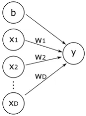
A neural network consists of interconnected processing units. A processing unit computes the output (activation)y=f(z) from external inputs (see Figure 2.1). f is called the activation function and z is calculated by mapping the inputs x1, ..., xD, weightsw1, ..., wDand biasbto the actual inputz. y=f(z) withz=

PD

i=1wixi+bi.

...

b

y x1

x2

xD

w1

w2

wD

Figure 2.1: A processing unit calculates the outputy=f(z) based on the inputs x1, ..., xD, weights w1, ..., wDand biasb.

Several activation functions could be used, which are discussed in paragraph 2.1.6.

A neural network contains multiple processing units, connected in several layers (see Figure 2.2). The first layer consists of input neurons, the final layer

of output neurons. The middle layers are called hidden layers. From one layer to the next, the neuron computes a weighted sum of all the input from the previous layer and passes the result through the activation function. yl

i=f(zil) withzil=

Pm

k=1w

l

i,ky

l−1

k +b

l

i The weights and biases of the network are trained using gradient descent (see section 3.1), to minimize a predefined cost function.

...

y(1)_m b(0)

x1

xD

...

y(1)₁

b(1) ...

...

... _y(L)_m

...

y(L)₁ b(L) 1st _{hidden layer L}th _{hidden layer} input layer ym ... y2 y1 output layer

Figure 2.2: Architecture of a multi-layer neural network. [2]

2.1.2

Convolutional layer

In a convolutional network the outputs of each layer form a feature map. The convolutional layer detects local conjunctions of features from the channels in a feature map [3]. A feature map is obtained by convolving the input channels with linear filters, one filter for each channel. The output of these convolutions are summed to form one channel in the output feature map. Multiple filter pairs are used, to extract different features from the input. This is illustrated in Figure 2.3. The feature map in layerLcontains four channels and is filtered by filterbank with two filters w1, w2 to the layer L+ 1, which contains two

channels. After the convolution operation, a bias term is added to the outputs of the convolution and an activation function is applied.

Denote the channels of a feature map withK channels as yk_{, k= 0..K and} i, j to the pixel location in the output feature map. The kth_{channel at layer l} is defined as yk(l)_{, the filter weights asw}k(l)_{, the biasb}k(l) _{and the activation}

functionf(.). The output channelyk(l)_{is now defined by:}

yk_ij(l)=f((wk(l)∗x)ij+bk(l))

The number of input channels differs for every layer. In the first layer the input is the image itself and the number of input channels depends on the color map. For example, grayscale images have one channel, RGB images three. In higher layers the number of input channels is equal to the number of different filters used in the previous layer. The weights wcan be represented as a 4D matrix, with shape [#filters, #input channels, filter width, filter height]. The weights of all the filters in every layer and the biases are trained using gradient descent (see Section 3.1).

There are three hyperparameters that define the convolutional layer: depth, stride and zero-padding. The depth refers to the number of filters pairs in the filterbank, each trained to look for something different in the input. In the example of Figure 2.3, the depth is two. The stride defines the step size in the

W31 W3

0 W32W33

W2 1 W2

0 W2

2W23 W11 W1

0 W12W13

W01 W0

0 W02W03

w1 w1

w2

w2

Layer L Layer L+1

Figure 2.3: Example of a convolutional layer. w1andw2filter different features

out of layerL, making the depth of the filterbank two. Image based on [4].

convolution operation. When a stride of one is used, the filters slide over the whole image, like normal 2D convolution. When the stride is two, the filters are moved two pixels at a time, jumping over the input image. This results in smaller output volumes. Zero-padding defines the number of zeros padded around the border before convolution. This enables the control of the spatial size of the output. The use of the convolution operator instead of matrix multiplication reduces the number of parameters to be trained, because the connectivities are sparse and the parameters shared. This is motivated by the idea that interesting features are repetitive and location invariant in the input data. The use of multiple layers allows to learn more complex structures from the input image.

2.1.3

Pooling layer

The pooling layer down-samples the input feature map by subsampling non-overlapping partitions of the input image to produce a single output. It provides a form of rotation and translation invariance. It reduces the dimensionality of the intermediate layers and therefore the number of parameters to be trained. Typically pooling is used, although other pooling operators exist. The max-pooling operator outputs the maximum value for non-overlapping partitions of the input image.

2.1.4

Fully-connected layer

After several convolutional and pooling layers, the output represents high-level features from the input image. To be able to learn non-linear combinations of these features, one or more fully-connected layers are added. In contrast to a convolutional layer, in a fully-connected layer every output is connected to all the input pixels as in classical neural networks. The output of the last fully-connected layer can be seen as an extracted feature vector of the input image.

2.1.5

Output layer

An output layer is added to the network and adds a final feature transformation. The output layer is again a fully connected layer, but with a different activation function. The choice of type of output unit is coupled with the choice of the cost function, in order to perform efficient training and prevent vanishing gradients. Classification problems with two classes can use the sigmoid activation function. The sigmoid function is defined as

σ(x) = 1 1 +e−x

The sigmoid function is often combined in training with the maximum log-likelihood, because it avoids saturation of the sigmoid [3]. When saturation occurs in gradient descent, the unit will not learn anymore, because the gradient approaches zero. The softmax function can be used to represent the probability distribution over n classes and can be seen as a generalization of the sigmoid function [3]. The softmax function is defined as

sof tmax(z)i= e

zi

P

jezj

Again training with the maximum log-likelihood works well, because the log undoes the exponential operation of the softmax. The negative log-likelihood cost function strongly penalizes the most active incorrect prediction [3].

2.1.6

Activation functions

Many types of activation functions are available. Traditional in neural net-works the logistic sigmoid activation function was often used, probably because sigmoids perform better when neural networks are very small [3]. However, the widespread saturation of the sigmoid function complicates gradient-based learning and therefore discourages the use of the sigmoid activation function in feed-forward networks. Currently the rectified linear unit (ReLU) [5] is one of the most popular activation functions [3], which behaves as a half-wave rectifier f(z) =max(z,0). Because of the linearity the gradient remains large whenever the node is active. The drawback is that the ReLU result in a zero gradient whenever the input is zero or less, making it impossible to learn via gradient descent. Therefore ReLU units could die and never become active again. Initial-izing the biases of the layer to a small positive value can improve the learning, because it is more likely for the ReLU to be initialized active, allowing the gradient to pass through [3].

There are several generalizations of the ReLU, which all use a non-zero slope

αi whenzi<0: fi(zi) =max(0, zi) +αimin(0, zi). Absolute value rectification

usesα=−1, resulting in the absolute value of the input. For a leaky ReLU [6] αi is fixed at a small value. αi is a learnable parameter for a parametric ReLU (PReLU) [7]. Maxout units divide the inputzinto groups ofkvalues, outputting the maximum element of one of these groups [8]:

f(x)i= max

j∈[1,k](zij)

wherezij =xTW...ij+bij with learned parameters. This can be interpreted as learning the activation function, by making a piecewise approximation.

Chapter 3

Training Convolutional

Networks

3.1

Gradient descent

Deep learning networks are commonly trained with gradient descent in com-bination with backpropagation and a cost function. The cost function val-ues the error in the current system. Backpropagation calculates the partial derivatives of the cost function and applies the chain rule to calculate the de-pendency between the cost and every parameter in the system. The parame-ters are updated every training cycle, using the learning rate and the partial derivative of the cost to every parameter. The CS231n lectures and lecture notes provide a good explanation of gradient descent and backpropagation; 1/ & http://cs231n.github.io/optimization-2/.

Ideally you want to calculate the loss combined for the whole training set together, in order to take the best step in parameter updates. However, this requires lots of computational power using the large datasets available today and slows down the learning process. Therefore Stochastic Gradient Descent is used which trains the network with batches from the training set. The training set is divided in mini-batches with a fixed size. The cost is calculated for all the samples in one batch. These costs are averaged and used to calculate the gradients for one parameter update. Thereafter a new batch is used for a new parameter update, until the whole training set has been passed. A single pass through all the samples in the training set, is called an epoch. The training is repeated several epochs, until the network converges. Before every epoch, the order of the samples in the training set should be shuffled. Otherwise the system will be trained on the same mini-batches every time, biasing the results and slowing down convergence.

Different cost functions can be used and the choice of the cost function relates to the type of output layer. Commonly used is the negative log-likelihood cost function C = −log(pt). Training highly depends on the initialization of the weights and biases. A commonly used initialization at the moment is the Xavier initialization [9]. The initialization scales with the number of parameters in a layer, in order to keep the variance constant. Practical recommendations for

training deep architectures with gradient descent, are given by Bengio in [10].

3.2

Regularization

When training a machine learning algorithm, it is important that it generalizes well on new data. Regularization strategies tend to reduce the generalization error but not the training error.

3.2.1

Weight decay

Weight decay adds penalty to the cost function, which depends on the parameter values and penalizes large weights, to reduce overfitting. Typically only the filter weights are penalized, regularizing the biases could lead to underfitting [3]. L2 weight decay adds a termλ1

2kwk 2 2=λ12

P

iw

2

i to the cost function, which causes the gradient to increase with a factor of the weight vector. λis a hyperparameter which controls the contribution of the weight decay. L1 _{weight decay adds} λkwk1 =Pi|wi|to the cost function. The gradient increases with a constant factorλwith a sign equal to sign(wi).

3.2.2

Early stopping

Early stopping uses a validation set, sampled from the training set, during training to evaluate when the networks starts to overfit and stop training after no improvement on the validation set for several time. The trained parameters that resulted in the lowest validation error are saved as final parameters. It can be seen as learning the training time hyperparameter.

3.2.3

Dropout

Dropout is a technique to prevents overfitting and approximates combining many different network architectures efficiently [11]. Units with their outgo-ing connections are temporarily removed (dropped) from the network, samploutgo-ing a thinned network from the total network (see Figure 3.1). The units that are dropped are chosen randomly with a probabilitypfor each new training case, from all the units except the output units. At test time all the weights are multiplied bypin order to remain the same expected outputs as in the training caseW_test(l) =pW(l)_{. Dropping connections from the network prevents the units}

to rely too much on other units. A hidden unit learns to work with randomly sampled connections, which makes the network more robust.

The authors mention one specific regularization technique that was especially useful for dropout, the max-norm regularization. In this case the norm of the incoming weight vector at each hidden unit is bounded by a constant c. The network is optimized under the constraintkwk2≤c. Goodfellow et al. designed

the maxout activation function to have beneficial characteristics for using in combination with dropout [8]. The ReLU uses the 0 in the max(0, z) activation function, which prevents the gradient from flowing through the unit in case of a negative activation and saturate. In Maxout units, the gradient always flows through every unit, even when it is 0, because this 0 is a function of parameters that may be adjusted.

Figure 3.1: Left: A standard neural network. Right: An example of a thinned network, using dropout. The crossed units and corresponding connections are removed. [11]

There are several variants of dropout, such as DropConnect [12] and DropAll [13] for example. These variants will not be further discussed here.

3.3

Additional techniques

There are some additional techniques used in training deep networks, which are found to enhance performances.

Data augmentation

Data augmentation is used to exploit the available training data. Popular is to horizontal flip the input images, take random crops or add color jittering. Other variations are manipulation of input images or constructing new images. Krizhevsky et al. [14] perform PCA on the RGB pixel values to change the intensities of the RGB channels in the training images.

Batch normalization

Batch normalization proposed by Ioffe and Szegedy [15] is a technique to nor-malize the input for every activation function, in order to keep the input closer to the expected input range. It applies whitening to the input of every inter-mediate layer and reduces the internal covariate shift. It is found to enhance performance and accelerate convergence. During training the statistics of the in-put data is captured and used for normalization. A running mean and variance is calculated to normalize the input (see Figure 3.2).

Extra techniques

Additional to the techniques discussed above, more optimizations are possible. Some of them are listed below with a reference towards the papers.

• Adaptive learning schedules - Adagrad [16], Adam [17]

• Hyperparameter optimization [18, 19]

• Momentum [20]

Figure 3.2: Pseudocode for the batch normalization algorithm [15].

Chapter 4

Convolutional Networks &

Face Recognition

Lots of research is done in the field of deep learning face recognition. A short overview of some well-known papers will be given below. The networks start with facial registration. Most of the networks use RGB images or a combina-tion with grayscale images. The number of convolucombina-tional, pooling and fully connected layers differs for every architectures. Some architectures train sepa-rate models for different faces regions. As explained in the paper, most networks train for multi-class classification and remove the classification layer to obtain a feature vector for verification.

DeepFace from Facebook [21] uses a tridimensional facial alignment, for rigid face registration in unconstrained scenarios. Their network architecture is shown in Figure 4.1 and uses locally-connected layers in the higher layers. They train for multi-class classification with a negative log-likelihood loss function and compare different similarity metrics, theχ2_{distance and a new-trained network.}

Face++ from Megvii trains convolutional networks for four different face regions (see Figure 4.4). The trained networks are 10 layers deep. The details of the networks are not provided. They achieve 99.50% accuracy on the LFW dataset. However, for in real-world application their accuracy is far from human level.

Sun et al. proposed several deep learning face architectures, based on each other; A hybrid architecture [24], DeepID [25], DeepID2 [26], DeepID2+ [27], DeepID3 [28]. They all contain a variant of the same basic convolutional network

Figure 4.1: Outline of the DeepFace architecture with locally connected layers in the higher layers (L4,L5,L6). They use two convolutional layers (C1, C3) and two fully connected layers (F7, F8). [21]

Figure 4.2: FaceNet learn with a triplet loss function to separate genuine and imposter pairs [22]

Figure 4.3: Network architecture used in FaceNet [22]

Figure 4.4: Convolutional networks are trained for four face regions in Face++ [23]

Figure 4.5: Variant of the basic network architecture used by Sun et al. [25]

(see Figure 4.5). All the architectures average networks trained for different face regions. DeepID2, DeepID2+ and DeepID3 embed verification signals into the loss function.

A comparison of different convolutional network implementation for face recognition is done by Hu et al in [29].

Chapter 5

Insight in Convolutional

Networks

Deep learning networks learn automatically to extract features from the input. Because multiple layers are cascaded, getting an insight into the working and learning process of the networks is not that straightforward. Several visualiza-tion methods for convoluvisualiza-tional networks are proposed in literature [30–32], of which one will be discussed in section 5.1.

The CS231n course explains clearly how to monitor the training process (see http://cs231n.github.io/neural-networks-3/). By plotting the cost and accuracy over the training time, the choice of learning rate and the amount of overfitting can be evaluated. The first layer of a network is relative easy to visualize, by showing the activations in a network during a forward pass or by visualizing the filter weights. For higher layers, these visualizations are somewhat harder to interpret. Showing the input images that maximally activates neurons gives an insight in what kind of inputs are important for the network. The same insight can be achieved by occluding parts of the images to see which occlusions change the output drastically.

5.1

Deconvolutional networks

Zeiler and Fergus propose to analyze convolutional networks by visualizing the activities of intermediate layers using deconvolutional networks [30]. This tech-niques reveals the input stimuli that cause activation in feature maps in any layer of the model. To analyze an activation in a specific layer an input image, which causes a high activation, is presented to the convolutional network and computed towards the output of every layer (the forward path). To analyze the given network activation the computed output in that layer is taken and all the other activations are set to zero. This single activation is presented to a deconvolutional network and propagated back toward the input pixel space (see Figure 5.1: Top). The deconvolutional network makes use of layers which unpool, rectify and filter the input activation, to reconstruct the activity in the layer below that caused this chosen activation.

The unpooling operation is a way to approximate the inverse of the max pooling operation. During the forward path, the locations of the maxima in the

Layer below pooled maps Feature maps Rectified feature maps

Pooled maps

Reconstruction Rectified unpooled maps

Unpooled maps Layer above reconstruction

Switches

Convolutional filtering Rectified linear function Max pooling

Max unpooling

Rectified linear function

Convolutional filtering

Figure 5.1: A deconvolutional layer (left) attached to a convolutional layer (right). The deconvolutional layer consists of unpooling, rectifying and filter operations. Image based on [30].

max pooling operation are saved into switch variables. These switch variables are used in the unpooling operation to place the reconstructions from the layer above in the appropriate locations (see Figure 5.2). The ReLU non-linearity rectifies the feature maps in the forward path. In the deconvolutional network the reconstructed signal is passed through a ReLU again to obtain a valid feature reconstruction. The filter operation in the deconvolutional network is used to inverse the filter operation of the forward path. Therefore it uses the transposed version of the filters of the forward path, which means simply flipping the filter horizontally and vertically. The use of these transposed filters act as a matched filter. The projections made by the deconvnets are not samples from the model but show the parts of the image that are discriminative.

Figure 5.2: The pooling operation results in the pooled maps and switch vari-ables, which saves the locations of the maxima. These switches are used in the unpooling operation. Image from [30].

Chapter 6

Practical Implementation

The network is implemented using the deep learning framework for Python, Theano [33]. A computer with Windows 7 64-bit Enterprise was used. The com-puter included 16GB RAM, a NVIDIA GTX 980 Ti graphics card and an Intel i5-2500 CPU. To install Theano, the manual provided on the Theano website was followed (see http://deeplearning.net/software/theano/install windows.html). We used Python version 3.4. Theano interfaces with the graphical card using CUDA. Our computer contains CUDA 6.5 combined with Visual Studio 2013. Interfacing with the correct versions of CUDA and Visual Studio is important in order to match the correct compilers. The manual for installing Theano let you make a bat-file to set the correct paths. These paths should be adjusted for the versions of software and compilers used. The bat-file used on our computer is shown in the code below. Other toolboxes are available but I chose Theano because it allows a lot of freedom in implementations. It is based on an easy to learn programming language (Python) and it runs on Windows.

REM configuration of paths

set VSFORPYTHON="C:\Program Files (x86)\Microsoft Visual Studio 12.0\VC" set SCISOFT=%~dp0

REM add tdm gcc stuff

set PATH=%SCISOFT%\TDM-GCC-64\bin;%SCISOFT%\TDM-GCC-64\x86_64-w64-mingw32\bin;%PATH%

REM add winpython stuff

CALL %SCISOFT%\WinPython-64bit-3.4.4.2\scripts\env.bat

REM configure path for msvc compilers

REM for a 32 bit installation change this line to REM CALL %VSFORPYTHON%\vcvarsall.bat

CALL %VSFORPYTHON%\vcvarsall.bat amd64

REM return a shell Spyder.exe /k

Preprocessing and normalizing the input data turned out to be important for the network performances. Without the normalized input data lot of filters became dead, probably because of the suppressed ReLUs. Normalizing the cost

function towards the subjects in the training set, improved the performance, when learning for multi-class classification. The training set should be shuffled before every training epoch, in order to train on different mini-batches every time and make training independent of the construction of the batches. Applying data augmentation in the training set by flipping the input images horizontally and changing the order of the image pairs was found to improve the performance. During the experiments in the earlier stage of the research the verification scores had a strong bias. The imposter scores had a wider range than the genuine scores. Using a dataset with more imposter than genuine pairs reduced this difference. In the final experiments we used equal number of genuine and imposter pairs in the dataset. It is interesting to investigate the influence of changing this ratio.

To answer the second research question, the dataset-sizes are differed in a controlled manner. A combination of twelve different public datasets is used, merged and used by Zeng et al. [34]. The number of subjects per sub-dataset is summarized in Table 6.1 in combination with Table 6.2.

Increasing images per subject

Dataset index 0 1 2 3 4 5 6 7 8 9 10 11

# Subjects per dataset 125 0 0 0 0 0 0 0 0 0 0 86

211 Subjects

Dataset index 0 1 2 3 4 5 6 7 8 9 10 11

# Subjects per dataset 12 0 1 0 0 2 0 9 0 4 0 183

422 Subjects

Dataset index 0 1 2 3 4 5 6 7 8 9 10 11

# Subjects per dataset 20 0 2 0 0 13 0 25 0 10 0 352

844 Subjects

Dataset index 0 1 2 3 4 5 6 7 8 9 10 11

# Subjects per dataset 49 0 5 0 0 28 1 49 0 24 0 688

1688 Subjects

Dataset index 0 1 2 3 4 5 6 7 8 9 10 11

# Subjects per dataset 99 0 5 0 0 42 1 95 0 37 0 1409

Table 6.1: Details on number of subjects per dataset, for dataset-size evaluation. Corresponding datasets are listed in Table 6.2.

Dataset Index

Multi-PIE [35] 0

PIE [36] 1

Pointing04 [37] 2

ORL [38] 3

AR [39] 4

Faces94 [40] 5

Grimace [41] 6

FRGC v2 [42] 7

FERET [43] 8

CAS-PEAR-R1 [44] 9

MUCT [45] 10

CASIA-WebFace [46] 11

Table 6.2: Datasets and their corresponding index in Table 6.1.

Bibliography

[1] Y. B. Ian Goodfellow and A. Courville, “Deep learning.” Book in prepara-tion for MIT Press, 2016.

[2] D. Stutz, “Understanding convolutional neural networks,” 2014.

[3] Y. LeCun, Y. Bengio, and G. Hinton, “Deep learning,”Nature, vol. 521, no. 7553, pp. 436–444, 2015.

[4] L. lab, “Convolutional neural networks (lenet).” http://deeplearning. net/tutorial/lenet.html. Accessed August 19, 2016.

[5] X. Glorot, A. Bordes, and Y. Bengio, “Deep sparse rectifier neural net-works.,” inAistats, vol. 15, p. 275, 2011.

[6] A. L. Maas, A. Y. Hannun, and A. Y. Ng, “Rectifier nonlinearities improve neural network acoustic models,” inProc. ICML, vol. 30, 2013.

[7] K. He, X. Zhang, S. Ren, and J. Sun, “Delving deep into rectifiers: Surpass-ing human-level performance on imagenet classification,” inProceedings of the IEEE International Conference on Computer Vision, pp. 1026–1034, 2015.

[8] I. J. Goodfellow, D. Warde-Farley, M. Mirza, A. C. Courville, and Y. Ben-gio, “Maxout networks.,”ICML (3), vol. 28, pp. 1319–1327, 2013.

[9] X. Glorot and Y. Bengio, “Understanding the difficulty of training deep feedforward neural networks.,” inAistats, vol. 9, pp. 249–256, 2010.

[10] Y. Bengio, “Practical recommendations for gradient-based training of deep architectures,” in Neural Networks: Tricks of the Trade, pp. 437–478, Springer, 2012.

[11] N. Srivastava, G. E. Hinton, A. Krizhevsky, I. Sutskever, and R. Salakhutdi-nov, “Dropout: a simple way to prevent neural networks from overfitting.,” Journal of Machine Learning Research, vol. 15, no. 1, pp. 1929–1958, 2014.

[12] L. Wan, M. Zeiler, S. Zhang, Y. L. Cun, and R. Fergus, “Regularization of neural networks using dropconnect,” inProceedings of the 30th Interna-tional Conference on Machine Learning (ICML-13), pp. 1058–1066, 2013.

[13] X. Fraz˜ao and L. A. Alexandre, “Dropall: Generalization of two convolu-tional neural network regularization methods,” inInternational Conference Image Analysis and Recognition, pp. 282–289, Springer, 2014.