University of Twente
TNO
Graduation Project
Extending the PowerMatcher using
Dynamic Programming
Student:
Y. Prins
Supervisors:
Dr. ir. W.R.W. Scheinhardt
Prof. dr. N.M. van Dijk
Prof. dr. J.L. Hurink
Dr. P.L. Kempker
Prof. dr. J.L. van den Berg
Abstract
The electricity grid did not change much over the last century. A few power plants are used to supply the electricity demand, whereby the power plants have to ensure that demand and supply of electra are always balanced. The transport of the electricity is realized via a layered network, and the flow of electricity is always from the highest layer, where also the power plants are con-nected, to the lower layers, where the customers are connected. Three important trends change the electricity network. Because of the increasing demand and supply of electricity and the decen-tralization of the electricity production, it becomes more difficult to balance electricity demand and supply. In the new situation electricity demand should follow the supply where possible. It is commonly believed that the current electricity network will no longer suffice and an intelligent electricity grid is needed to deal with the changes.
One of the technologies to support the intelligent grid is the PowerMatcher, which is introduced by a group of international partners. It is designed to match current demand and current supply and uses a lot of renewable energy in doing so. The current version of the PowerMatcher has some weaknesses and can therefore be improved. One way to do this is to not only use the current demand and current supply but also predictions about future demand and future supply. An attempt to integrate these predictions has led to the two-time-scale PowerMatcher, an extension of the PowerMatcher.
1 Introduction . . . 4
2 Background and literature . . . 5
3 The PowerMatcher . . . 8
3.1 The standard PowerMatcher . . . 8
3.2 Planning modules for the PowerMatcher . . . 10
3.3 Bidding strategies and bidding curves . . . 12
3.4 Research Question . . . 13
3.5 Outline . . . 14
4 Two-time-scale PowerMatcher . . . 15
4.1 Assumptions and frequently used variables . . . 15
4.2 Two-time-scale PowerMatcher algorithm . . . 15
4.3 Bidding strategies and curves in the two-time-scale PowerMatcher . . . 17
4.4 Advantage two-time-scale PowerMatcher over ‘simple’ strategies . . . 19
5 Bidding strategies using Dynamic Programming . . . 23
5.1 Determine price distribution . . . 24
5.2 DP using known prices . . . 27
5.3 DP using price distributions . . . 29
5.4 Extension to different appliances . . . 31
5.5 Updating prices . . . 33
5.6 Conclusion . . . 33
6 Results . . . 34
6.1 Advantage two-time-scale PowerMatcher over ‘simple’ strategies . . . 34
6.2 Bidding strategies using dynamic programming . . . 40
6.3 Compare different bidding strategies . . . 43
7 Conclusions and Further Research . . . 54
7.1 Conclusions . . . 54
7.2 Remarks and further research . . . 55
8 References . . . 56
1. INTRODUCTION
1
Introduction
Energy plays an increasingly important role in many aspects of our life. Electricity is used for lighting and cooling while fuel is used for transportation and heating. Our production and use of energy contributes for a large part to the climate change. Because of the thinning ozone layer, global warming and sea-level rise, environmentally friendly forms of power generation are asked for. The last years a lot of effort and research is put into different environmentally friendly power generation types. Wind and solar power are two examples of these power generation types, which are used more and more in the last years. The number of households that have a solar panel on their rooftop and the number of wind parks offshore increases. In the Netherlands, the aim is to provide at least 1 million households with energy from these wind farms, [17].
Because of these new types of power generation and the ability of households to produce small amounts of energy, the power grids are changing. Instead of power flowing from a few large power plants to a lot of small consumers, power will now flow both ways. Also, energy from renewable resources fluctuate in availability. Keeping the power supply and demand balanced is becoming a challenge through this change. Because of the flexibility on the supply side, also more flexibility on the demand side is needed. The current power grids are not able to manage these new kinds of energy generation and its flexibility. An intelligent system is needed to deal with the new kinds of energy generation and to prevent the grid from overloading, a smart power grid is needed.
An important component of this smart grid is demand-side management. Demand-side man-agement is used to reduce the peak electricity demand. This is where the PowerMatcher comes in. The PowerMatcher is a smart grid technology, developed by TNO together with industry and research partners, that matches energy supply and demand and uses a lot of renewable energy in doing so, without overloading the power grid. The idea behind the PowerMatcher is that every producing and/or consuming device sends a bidding curve which shows the willingness to pay for different electricity prices. These bidding curves are made using a certain bidding strategy and show the electricity demand at each price. This demand is negative when electricity is generated and positive when electricity is consumed. The electricity supply and demand can be balanced by putting all these bidding curves together.
The PowerMatcher uses current demand and current supply, where the generated amount of elec-tricity from renewable energy resources is dependent on the availability of wind/solar radiation. It would be great to know the wind/solar radiation availability in advance, planning could then be used to improve the PowerMatcher. The availability of wind/solar radiation is however not known in advance, forecasts about wind/solar radiation availability are accessible. Planning, based on the forecasts, could still improve the PowerMatcher. Whether this improvement is possible depends for a large part on the quality of the forecasts. Bad forecasts give a wrong idea about the future, which leads to bad decisions. Good forecasts can have an added value to the PowerMatcher and its bidding strategies, depending on how the information is used. The question arises whether an inclusion of the forecasts indeed improves the PowerMatcher and how wind/solar radiation fore-casts have to be included into the PowerMatcher. These questions will be studied in this report.
2
Background and literature
Electricity is one of the most widely used forms of energy. It is a secondary energy source and is generated from other sources of primary energy, like coal, natural gas and oil, at a few large power plants. Because electricity is generated from primary energy sources, electricity demand can be seen as energy demand. The terms ‘electricity demand’ and ‘energy demand’ will therefore be used interchangeably in this report and have the same meaning.
An electricity grid is an interconnected network where electricity is delivered from producers to consumers. The electricity network did not change much over the last century and depends on large power plants. These few power plants generate electricity which is transported to many consumers all over the country via the electricity grid. The electricity grid is divided into different voltage levels. The electricity generated at the power plants flows into the network at the high voltage level. The voltage level is lowered when the electricity is closer to the customer, this is done using transformers. Finally, the electricity is delivered to the customer via the low voltage distribution grid. Electricity can also flow into the network at lower voltage levels, this electricity is mostly generated from renewable energy sources. This type of inflow has increased in the last years, together with the generation of electricity from renewable sources.
The electricity grid differs from a lot of other networks (e.g. road networks) by the fact that the production and consumption needs to be balanced at all times. Since the network itself has no storage capacity and the consumers do not want to wait for the needed electricity, the generation of electricity is demand driven. As a consequence of the liberalization of the electricity markets, the production, transportation and distribution of electricity is carried out by different independent companies. The production companies own the power plants and generate the electricity, there are multiple production companies that have to compete with each other. The transportation companies own and maintain part of the electricity grid without any competitors. The distribu-tion companies sell the electricity to the customers, these companies have to predict the amount of electricity their customers will use and have to buy this amount from production companies. The distribution companies try to predict the consumption of electricity as accurately as possible to prevent penalties due to imbalance.
There are currently three important trends in the electricity system [1]. These are listed below.
• Demand of electricity increases every year and is expected to keep increasing in the coming years. The electrification of everything leads to this rise in demand. This rise in electricity demand will drive the distribution networks to their capacity limits. Overloading the grid will shorten the life span of the networks, which are already close to their life end.
• Supply of electricity increases and becomes more uncontrollable and unpredictable. More electricity is generated from renewable energy resources, the availability of energy from renewable resources is dependent on the availability of wind/solar radiation. The increased and more unpredictable amount of energy supply makes it harder to balance the supply and demand of electricity.
• The electricity production is becoming more and more decentralised. The number of wind turbines and solar panels has increased and is expected to keep increasing in the coming years. This increase changes the electricity system, the electricity system is now based on a few large power plants and will in the near future be based on many small producers.
2. BACKGROUND AND LITERATURE
smart grid is defined in [4] as an electric system that uses information, two-way, cyber-secure com-munication technologies, and computational intelligence in an integrated fashion across electricity generation, transmission, substations, distribution and consumption to achieve a system that is clean, safe, secure, reliable, resilient, efficient and sustainable.
Demand-side management will be an essential part in the smart grid. Traditionally, power plants adjust the power generation to meet the rising demand, demand-side management (DSM) will look at the other side, the demand of electricity. DSM encourages consumers to use less energy during peak hours or to move the time of energy use to off-peak hours, see [13]. This encouragement is needed because the peak loads are increasing. The evening peak, for example, will increase because of the increasing amount of plug-in hybrid vehicles that are charged after working hours. The impact and opportunities for the electricity grid with this increasing amount of plug-in hy-brid vehicles is studied in the European project: Grid-for-Vehicles (G4V), see [20]. This G4V project has, among others, studied the peak load in the grid using different scenarios, see [14]. Several solutions for DSM of plug-in hybrid vehicles are given in [18]. These solutions do all take advantage of the two-way communications. Another DSM system that takes advantage of the two-way communication infrastructure is given in [12]. In [12] game theory is used and an energy consumption scheduling game is formulated. The players in this game are the electricity users and their strategies are the daily schedules of their household appliances and loads. Game theory is a study of mathematical models of complex interactions between intelligent rational decision makers. In [15] an overview of the potential of applying game theory within smart grid systems is given. Besides [18] and [12], other demand-side management systems are looked at in the last years. A few of these systems are given in [16]. A smart management system is however not enough to create a smart grid, a smart infrastructure and protection system is also needed. A few infrastructure and protection systems are given in [3].
There are many ongoing projects to create a smart grid, see [5]. One of the technologies to support the smart grid is called the PowerMatcher. The PowerMatcher, [10], is a smart grid technology created by TNO in cooperation with industry and research partners. In the Power-Matcher, users determine their bidding curve, which is a curve showing the electricity demand of the user at different electricity prices. These bidding curves are determined using a certain strat-egy, knowledge about the average price is used to determine this bidding strategy. The bidding curves are used in the PowerMatcher to balance the total supply and total demand. By balancing the total supply and total demand, the PowerMatcher automatically determines the amount of produced/consumed electricity of each user.
The “capability” of the PowerMatcher to support the mass integration of electricity produced by wind energy has been studied in [11]. More precisely, the goal in this research was to adapt flexible household demand and supply to the availability of wind power. The need for fossil fuel based electricity will, in this way, be reduced.
The PowerMatcher can be improved and extended. In the current version of the PowerMatcher the average price is used by the user to determine the bidding strategy. When besides the average price also forecasts about future prices are known, planning can be included in the PowerMatcher. One extension of the standard PowerMatcher is therefore a combination of two instances of the PowerMatcher, the two-time-scale PowerMatcher, see [7]. These two instances operate on different time scales. With these two instances it is intended to make decisions about short term demand using information about the long term, which may lead to more cost-efficient schedules. Whether the two-time-scale PowerMatcher improves the PowerMatcher depends to a large extent on the quality of the long term information.
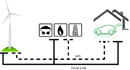
Why demand-side management is needed and where the two-time-scale PowerMatcher comes in can be shown using a small example network. This network, see Figure 2.1, consists of one wind-mill, one household with an electric car and flexible energy resources. Energy generated by the windmill is cheaper than the energy produced by flexible energy resources, but wind energy is not always available while energy from flexible energy resources is.
Figure 2.1: Network with one windmill and one household with an electric car
The energy demand of the electric car is shiftable over a long time period. The question arises when the electric car has to be charged to minimize the costs of charging the car. Without any communication and information about future demand, the car is charged as soon as pos-sible. This may lead to high costs and a high amount of energy generated by flexible energy resources. To lower the costs demand-side management is needed, demand-side management is used to match the wind energy and the car’s demand. Using communication and information about future demand, the two-time-scale PowerMatcher tries to create a situation where a lot of available renewable energy and a minimal amount of energy from flexible energy resources is used. This report tries to improve the two-time-scale PowerMatcher in order to reduce the total amount of energy used from flexible energy resources and the total costs of satisfying the shiftable demand.
3. THE POWERMATCHER
3
The PowerMatcher
This report will look at the bidding strategies used in the PowerMatcher. Before looking at the bidding strategies, first the PowerMatcher has to be explained. The standard PowerMatcher is described in Section 3.1. This PowerMatcher can however be improved. One possible way to do this is to extend the PowerMatcher to the scale PowerMatcher, this two-time-scale PowerMatcher is introduced in Section 3.2. In both versions of the PowerMatcher bidding strategies are used. Section 3.3 explains how, where and which bidding strategies are used in both versions of the PowerMatcher. With information about the standard PowerMatcher, two-time-scale PowerMatcher and bidding strategies, the research question can be given, the research question is given in Section 3.4.
3.1
The standard PowerMatcher
The electricity network is changing. The electricity demand and supply are increasing and more renewable energy becomes available. Sufficient management is needed to prevent the grid from overloading. The PowerMatcher, [10], is one of the technologies to match energy demand and supply, using available renewable energy and preventing the grid from overloading.
Systems design of the PowerMatcher
Within a PowerMatcher cluster agents are organized into a tree. The agents are the producers and consumers of electricity and are represented by the leafs of the tree, these agents are also called local device agents. One of the leafs could be an objective agent. There is also an auctioneer agent, at the root of the tree. The auctioneer agent is a unique agent that handles the price forming. In order to obtain scalability, concentrator agents can be added to the structure as tree nodes. Figure 3.1 shows an example PowerMatcher agent cluster.
The different agent types are described in [10] and are repeated below:
• Local device agent: This agent is the representative of a DER device. The local device agent coordinates its actions with all other agents in the cluster by buying or selling electricity. The agent communicates its latest bidding curve to the auctioneer agent and receives price updates from the auctioneer agent. The latest bidding curve and the current price determine the amount of electricity the local device agent is obligated to produce or consume.
• Auctioneer agent: This agent determines the price. The auctioneer agent receives the bidding curves of all agents and searches for the equilibrium price. The agent communicates the equilibrium price back to all agents.
• Concentrator agent: The concentrator agent represents a sub-cluster of local device agents. The agent concentrates the market bidding curves of the agents in the sub-cluster and aggregates this into one bidding curve. The agent then communicates this curve to the auctioneer agent. The agent also communicates the price, received from the auctioneer agent, to all local device agents in the sub-cluster. The concentrator agents look like the auctioneer agent from the perspective of the local device agents in the sub-cluster.
• Objective agent: The objective agent gives the cluster its purpose. When the objective agent is absent, the goal of the cluster is to balance itself. Depending on the specific application, the goal of the cluster might be different. If the cluster has to operate as a virtual power plant, for example, it needs to follow a certain externally provided setpoint schedule. The externally imposed objective can be realized by implementing an objective agent.
All agents, except the auctioneer agent, send a bidding curve to the higher agent. This bidding curve shows the electricity demand at each price. The bidding curve is explained in more de-tail in Section 3.3. The auctioneer agent receives all these bidding curves and determines the corresponding price. This price is send back to all agents.
Structure of the PowerMatcher
The structure of the PowerMatcher is given in Figure 3.2. A certain time scale is used in the PowerMatcher, in this figure the hour scale is used. So agents send a bidding curve every hour. This time scale can however be chosen differently, agents could for example sent a bidding curve every 15 minutes.
3. THE POWERMATCHER
In this figure, agentkrepresents one of the many agents in the tree. The steps in the PowerMatcher algorithm are given below:
• The PowerMatcher algorithm starts at the bottom, where the agent determines the bidding strategy over the next hour. The bidding curve corresponding to this strategy shows the demand,dk, the agent is willing to buy or sell at each price,p.
• All agents (leafs in the tree) make such a bidding curve and send this curve to the next higher agent.
• The next-higher agent aggregates the received bidding curves and passes them on. Finally the combined curve,dtotal, reaches the root.
• The root determines the price,p∗, over the next hour such thatdtotal equals zero (then the supply and demand of electricity are the same).
• Thisp∗ is sent back to all agents and each agent knows the demand it must buy or sell,d∗k.
• An hour later, tbecomes t+ 1 and the whole process is repeated.
Sending a bidding curve with a higher/lower electricity demand at each price leads to higher/lower prices which could be advantageous for producers/consumers. It is therefore assumed that agents do not lie about their bidding curve.
3.2
Planning modules for the PowerMatcher
The PowerMatcher algorithm developed in [10] balances the short-term supply and demand in the smart grid. This is done while taking the network capacity constraints into account. The bidding curve corresponding to the agent’s bidding strategy is made every fixed time unit, without any forecasts about future prices. Historical data may be available but this is not a good indication of future prices if wind energy is involved. To make more efficient choices, it would for some devices be better to know the long-term price expectations and use this information into their bidding strategy. For devices which are shiftable over a longer time window than the chosen one, it is beneficial to know the lowest prices within that longer time window. One way to predict the long-term price is to use weather forecasts. Including the long-term price predictions into the PowerMatcher may lead to a more cost-efficient schedule for shiftable devices.
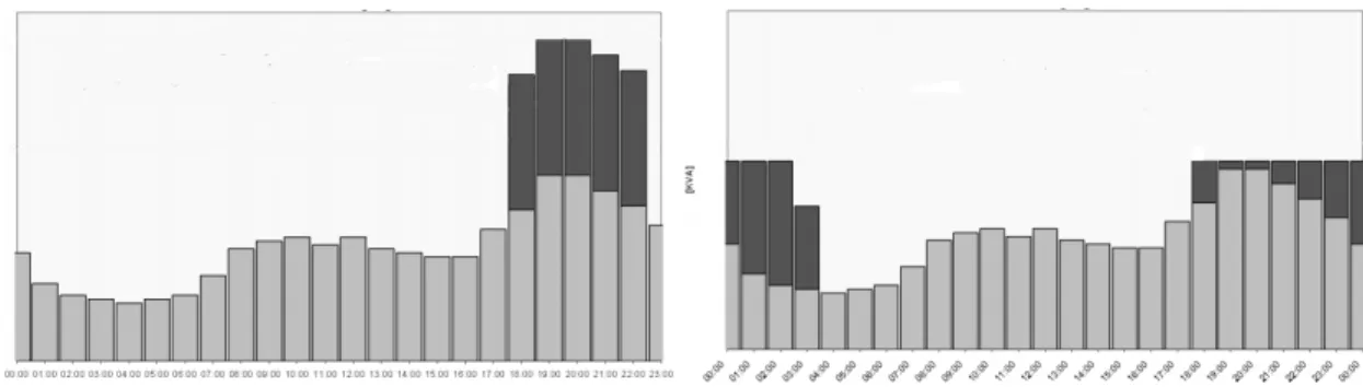
To show the potential of including planning modules, a small example is used. Suppose that there are a few electric cars that have to be charged between 18.00 and 08.00 the next day and that an electric car can be charged in five hours if it is charged at full power. Without any plan-ning, all cars start charging at full power at 18.00 . This situation is shown in Figure 3.3. All cars are fully charged at 23.00.
Figure 3.4 shows another way to handle the increasing amount of needed electricity. With con-trolled charging possible network overloading is avoided. This is also what the standard Power-Matcher does, the standard PowerPower-Matcher tries to control the charging of electric cars to avoid the network from overloading.
There is still room for improvement. The electric cars need to be fully charged at 08.00. As can be seen from Figure 3.4 the electric cars are already fully charged at 04.00. This means that the cars could be charged slower. By taking planning into account the load can be divided more evenly over the night and the peak load of electricity in the network decreases. The network will in that case be far from overloading. This situation is shown in Figure 3.5. The gap between 04.00
Figure 3.5: Controlled charging using time till 08.00
and 08.00 is filled, it is expected that this leads to lower overall costs. This last case can only be achieved when information about future demands is known. Matching future demands leads to future price expectations.
There are different options for including planning in the PowerMatcher, one of them is the two-time-scale PowerMatcher, [8]. The two-two-time-scale PowerMatcher charges the electric cars with information about future demands/prices and remaining time. This is done using different time scales. The longer time scale is needed to get information about future demands/prices and the shorter time scale is needed to match demand and supply over the shorter time scale.
In the example above the two time scales used by the two-time-scale PowerMatcher would be the day-ahead scale and the hour scale.
• Day-ahead scale: Agents send their bidding curve over the whole day and an average price is constructed from these curves. This average price can be used to determine the bidding curve for the shorter time scale.
• Hour scale: With the information about the expected average price, agents construct their bidding curve for the next hour. The price for the next hour is determined using the short term bidding curves of all agents.
3. THE POWERMATCHER
Systems design of the two-time-scale PowerMatcher
The systems design of the two-time-scale PowerMatcher is the same as the systems design of the PowerMatcher using one time scale. Within a cluster, agents are organized into a tree. The layout of this cluster is given in Figure 3.1 in Section 3.1, where the different types of agents are also described.
Structure of the two-time-scale PowerMatcher
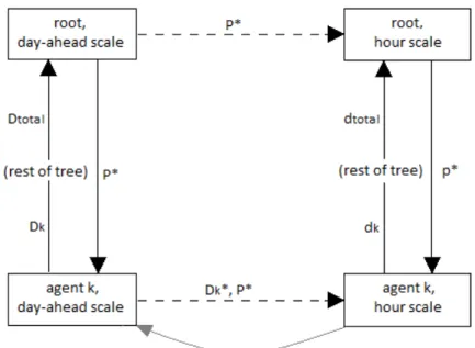
The structure of the two-time-scale PowerMatcher is given in Figure 3.6. In this figure the day-ahead scale and the hour scale are used.
Figure 3.6: Structure two-time-scale PowerMatcher
The right side of Figure 3.6 is equal to Figure 3.2, the two-time-scale PowerMatcher does however start at the bottom left node. Agents determine the day-ahead bidding curve and send this curve to the next-higher agent. By aggregating the different bidding curves, the total bidding curve
Dtotal reaches the highest agent/root. This root determines the the day-ahead average price,P∗, and sends this price back to all agents. WithP∗ known, agents can determine the bidding curve for the shorter time scale. This happens at the right side of Figure 3.6. This right side works exactly the same as explained in Section 3.1, but withP∗ as extra information. A more detailed description of the structure of the two-time-scale PowerMatcher is given in Section 4.2.
3.3
Bidding strategies and bidding curves
Above, the PowerMatcher is explained. In the PowerMatcher there are different agents. These agents have to determine their bidding strategy and make the corresponding bidding curve. In the standard PowerMatcher one bidding curve has to be sent at each time epoch, the bidding curve over the next time interval. In the two-time-scale PowerMatcher each agent has to sent two bidding curves, one bidding curve over the longer time scale and one over the shorter time scale.
a lot of different bidding strategies possible. Agents can use aggressive and passive bidding strate-gies. Aggressive bidding strategies have a high demand at very low prices and a very low demand when prices are higher. Passive bidding strategies use more demand at higher prices, compared to the aggressive bidding strategies. Aggressive bidding strategies lead to steeper bidding curves.
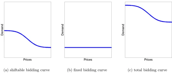
There are different kinds of demand, some fixed and some shiftable. Fixed demand has to be satisfied at each price, this is not the case with shiftable demand. The amount of shiftable de-mand at a certain time depends on the price. At a low price the shiftable dede-mand will be high, the demand can be satisfied at a relatively low price. With the same reasoning, the shiftable demand will be low at a high price. The bidding curve that is send to the higher agent is the summation of the bidding curves per demand type. An example of this is given in Figure 3.7. Suppose that an agent has a fixed and a shiftable demand. The total bidding curve is the summation of the bidding curves of these two different demand types.
(a) shiftable bidding curve (b) fixed bidding curve (c) total bidding curve
Figure 3.7: Agent’s fixed and shiftable demand bidding curve is summated to one bidding curve
The fixed demand is the same for each price. The bidding curve for the fixed demand is therefore a straight line. The shiftable demand can be different at each price, the amount of demand at each price depends on the bidding strategy.
Each agent sends a bidding curve at each time epoch. These bidding curves are different for each agent and each time epoch. Each agent wants to fulfill the demand as cheaply as possible, but each bidding strategy leads to different total costs. A few different bidding strategies are looked at in the remainder of this report, these bidding strategies will be compared to each other by looking at the total costs for satisfying a certain amount of demand.
3.4
Research Question
This section summarizes the background and states the research question.
Due to the growing energy needs and larger shares of decentralized and renewable energy, smart control algorithms play an increasing role in the energy field. For the coordinated matching of supply and demand in the electricity network, TNO (together with ECN) developed the Power-Matcher. The PowerMatcher is a coordination mechanism that balances short term demand and short term supply in large clusters of distributed energy resources.
3. THE POWERMATCHER
need information about the long-term price expectations. These price expectations can be ob-tained by producing demand forecasts, based on the individual demand predictions of the device agents. This extension of the PowerMatcher is called the two-time-scale PowerMatcher.
The question arises whether this extension to a two-time-scale PowerMatcher provides an added value to the PowerMatcher and how the price expectations have to be included in the bidding strategies of the two-time-scale PowerMatcher. The research question reads therefore:
• Does the performance of the PowerMatcher improve when next to the current demand and current supply also predictions about future demand and future supply are included in the planning and to which extent does the performance improve?
• How should predictions about future demand and future supply be included in the bidding strategies of the two-time-scale PowerMatcher?
3.5
Outline
4
Two-time-scale PowerMatcher
As stated before, the main goal of this report is to improve the PowerMatcher by not only using current demand and current supply but also predictions about future demand and future supply. Extending the standard PowerMatcher to the two-time-scale PowerMatcher is one of the methods to include planning into the PowerMatcher. This two-time-scale PowerMatcher is already shortly introduced in Chapter 3 and will be explained in more detail in this chapter.
First, in Section 4.1 the assumptions are given under which the two-time-scale PowerMatcher is worked with in the report. Also the most frequently used variables are given in this section. The two-time-scale PowerMatcher algorithm, as developed in [8], will be given in Section 4.2. In this algorithm bidding curves have to be sent by the agents, the agents’ bidding strategies and curves in the two-time-scale PowerMatcher are explained in Section 4.3. The bidding strategy used in Section 4.2 is compared to two other demand satisfying strategies in Section 4.4. These two strategies do not have information about future demand and supply.
A new bidding strategy will be introduced in the next chapter. This new bidding strategy will be compared to the bidding strategy explained in Section 4.3, this to see if the current version of the two-time-scale PowerMatcher can be improved.
4.1
Assumptions and frequently used variables
A few assumptions are made throughout this report. These assumptions are listed below.
• It is assumed that agents send a bidding strategy once in every fixed amount of time. This is not what happens in real life. To keep the communication between the agents to a minimum, new bidding strategies are only sent when the local device state changes. Sending new bidding strategies is thus event-based in practice.
• It is possible for agents to lie about their needed demand at a certain price. Producers want to raise the price of energy to earn more, consumers like a low price. By changing the real bidding curve, agents can influence the price to their own benefit. It is assumed in this report that agents play fair.
• It is assumed in this report that there are no storage units. Producers can not store produced energy, to sell it later at a higher price, and consumers can not store bought energy, to use it at another time.
• The information about future prices is in this report based on weather forecasts. Information from the past is not used.
• The prices of two consecutive time periods are independent, the price can thus fluctuate heavily.
• It is assumed that all demand is shiftable, unless stated otherwise.
Some frequently used variables in this section are listed in Table 4.1. A list of all used variables in this report is given in Table 9.1.
4.2
Two-time-scale PowerMatcher algorithm
This section gives the algorithm of the two-time-scale PowerMatcher. The algorithm shows among others when the bidding curves are made and what information is used by the agent to make a bidding curve. The algorithm also shows how the prices are determined.
4. TWO-TIME-SCALE POWERMATCHER
Variable Description
t time (measured in intervals of hours), short time scale
nt number of time points
T time horizon, long time scale
K number of agents
d demand at shorter time scale
D demand at longer time scale
p unit price of energy at shorter time scale
P unit price of energy at longer time scale
Table 4.1: Frequently used variables
steps which will all be looked at. The two time scales worked with here will be the hour scale and the day-ahead scale. These two time scales are also mentioned in Figure 3.6.
1. The starting node is the node “agent k, day ahead scale” at the beginning of time t. The day-ahead horizon is denoted byT,T = [t, . . . , t+nt].
2. Agent k, k ∈ K, determines the bidding strategy over T and creates the bidding curve
Dk(P;T) over T, where P is the price. The demand may depend on the average price,
P∗ overT but this is only possible when the demand is shiftable over a longer time period than T. When no shiftable demand is available or if the shiftable demand is only shiftable withinT, the agent’s demand will be constant and therefore independent ofP∗. The bidding strategy of the agent is explained in Section 4.3.
3. Agentk sendsDk(P;T) to the next-higher agent in the tree.
4. Each agent in the tree aggregates the received information (bidding curves) and passes it on to the next-higher agent in the tree. Finally, Dtotal(P;T) reaches the root.
Dtotal(P;T) = K
X
k=1
Dk(P;T).
5. The root finds the average price,P∗, such that the total bidding curve atP∗ equals zero.
Dtotal(P∗;T) = 0.
Arguments for the existence and uniqueness of the solution P∗ can be found in [10].
6. P∗ is the new day-ahead average price. This value is sent to all agents in the tree.
7. By plugging inP∗intoDk(P;T), agentknow knows it’s target demand over the day-ahead horizon.
D∗k=Dk(P∗;T).
8. Agentkcan useP∗andD∗
kas inputs for the bidding curve over the next hour,dk(p;t|D∗k, P∗). This dk(p;t, d|Dk∗, P
∗) corresponds to the agent’s bidding strategy over the next hour. The
bidding curvedk(p;t, d|D∗k, P
∗) consists of different kinds of demand, see Section 3.3.
9. Agentk sends the bidding curvedk(p;t|Dk∗, P∗) to the next-higher agent in the tree.
10. Each agent in the tree aggregates the received information (curves) and passes it on to the next-higher agent in the tree. Finally the combined curve dtotal(p;t|{D∗k}k=1,...,K, P∗) reaches the root. The dtotal(p;t|{Dk∗}k=1,...,K, P∗) equals the sum of all agents’ hourly de-mand.
dtotal(p;t|D∗k, P∗) = K
X
k=1
11. The root finds the price,p∗, such that the total demand atp∗equals zero.
dtotal(p∗;t|Dk∗, P∗) = 0.
12. The current price is equal top∗, this price is sent to all agents in the tree.
13. Agentk can putp∗, intodk(p;t|Dk∗, P∗). The resulting demand,d∗k is binding.
d∗k =dk(p∗;t|Dk∗, P∗).
14. An hour later,tbecomest+ 1, the time horizonT gets shifted by one period and the whole algorithm is repeated.
The dk(p;t|Dk∗, P∗) are made with the knowledge of D∗k and P∗, this does not mean that the total demand and real average price equal these values determined at the beginning. It turns out that these values differ most of the time. One way by which D∗k and P∗ differ from the total demand and real average price is when producers can’t deliver the amount of electricity given in the bidding curve. When the total demand of all agents is positive, electricity has to be bought from expensive but flexible energy resources. When the total demand is negative, energy is thrown away.
4.3
Bidding strategies and curves in the two-time-scale PowerMatcher
Bidding strategies have to be made for the shorter and longer time scale in the two-time-scale PowerMatcher, as explained in Section 4.2. This section explains the bidding strategies for the shorter time scale. The idea behind the bidding strategies for the longer time scale is the same, but without the information aboutD∗t andP∗.
The bidding strategy gives the method used to determine the bidding curve and the bidding curve shows the demand at each price. The bidding curve of agentk,dk(p;t, d), is dependent on pricepand can be different for each time epoch t and remaining demandd. The bidding curve currently made in the two-time-scale PowerMatcher is however independent of d. The bidding curve of agentk will in this section therefore be denoted bydk(p;t). Later on in this report the bidding curve will be dependent ofd.
The bidding curve dk(p;t) would ideally show the demand at each p. The price p is however continuous and it is therefore very hard to determine the demand for each value of p. To deal with thisdk(p;t) will be a piecewise linear function,n possible values ofp, r1, ..., rn are selected betweenpmin andpmaxand the corresponding action/demandak(r1;t), .., ak(rn;t) is determined such that agent k satisfies the total demand as cheaply as possible. The values of r1 and rn are fixed, r1 = pmin and rn = pmax. The combinations ri and ak(ri;t) for i = 1, ..., n are the breakpoints of the piecewise linear function. The breakpoints of the function are given in a nx2 matrix.
r1 ak(r1;t)
..
. ...
rn ak(rn;t).
.
An agent can have different kinds of demand, fixed and shiftable demand and also demand from wind and flexible energy resources are possible. Each kind of demand has its own bidding strategy. The first two demand types are positive while the last two are negative. The four different demand types and bidding strategies are explained next.
The fixed demand,dk,f ixed(t), is an amount which has to be satisfied at timet, sop,Dk∗ andP∗
do not have any influence on this value, i.e. dk,f ixed(t) is a fixed amount,d f ixed k,f ixed(t).
4. TWO-TIME-SCALE POWERMATCHER
The shiftable demand, dk,shif t(p;t|Dk∗, P∗), does depend on pand P∗. It would be beneficial to satisfy a lot of shiftable demand when pis low and to use no shiftable demand when p is very high. Ifp=P∗ for allt, the total shiftable demand at timet, d
k,shif t total(t), would be satisfied equally overt.
dk,shif t(P∗;t|Dk∗, P∗) = dk,shif t total(t)
T−t+ 1 .
Most of the timesp6=P∗, a possible bidding strategy for shiftable demand is given below.
dk,shif t(p;t|D∗k, P∗) =
dk,shif t total(t)·
1 +(p p min−P∗)·
1− 1
T−t+1
if p≤P∗ dk,shif t total(t)
T−t+1 if p = P
∗
0 if p≥P∗
.
Whenp=P∗, dk,shif t total(t) is divided over the remaining times equally and the part assigned to time t is satisfied. When p≥P∗, no shiftable demand will be satisfied. When p≤ P∗, the amount of satisfied shiftable demand depends on the value ofp. The functiondk,shif t(p;t|p≤P∗) is a linear function wheredk,shif t(pmin;t|D∗k, P∗) =dk,shif t total(t) anddk,shif t(P∗;t|D∗k, P∗) is as given above, one t’th part of thedk,shif t total(t). The given bidding strategy for shiftable demand is currently used in the two-time-scale PowerMatcher. There are however more bidding strategies possible, agents can choosedk,shif t(p;t|Dk∗, P∗) however they want.
The demand of a wind turbine,dk,wind(p;t) does not depend onp, it only depends on the available amount of wind. The wind demand is therefore fixed.
dk,wind(t) = −d f ixed k,wind(t).
An agent with storage options can choose to store part of the df ixedk,wind(t). This part could then become available at another time. It is assumed in the beginning of this chapter that this is not possible in this report.
Another type of demand is the demand from a flexible energy resource, like a diesel genera-tor. The bidding curve of a diesel generator,dk,diesel(p;t), is independent ofP∗, the bidding curve depends entirely on the price of power generation. dk,diesel(p;t) is given below. Here, the unit cost of generation is denoted byπg. So, forp>πg the agent with the diesel generator can make profit and will therefore produce as much as possible, dmaxk,diesel. Whenp<πg, the diesel generator will not produce anything.
dk,diesel(p;t) =
0 if p(t)
≤πg
−dmax
k,diesel if p(t) > πg
.
When agent krepresents a household where the total demand consists of fixed and shiftable de-mand, the bidding curves of the fixed and shiftable dede-mand,dk,f ixed(t) anddk,shif t(p;t|D∗k, P∗), are added, as explained in Section 3.3.
dk(p;t|Dk∗, P∗) = dk,f ixed(t) +dk,shif t(p;t|D∗k, P∗).
Agentkwants to get the total demand as cheaply as possible and therefore wants to choosedk(p;t) such that the costs are minimized. Thedk,f ixedis fixed and there is therefore not much to choose,
dk,shif tis not fixed and therefore can be chosen by the agent. The goal is now to choose the best one, the one that minimizes the total costs.
Thedk,shif t(p;t) currently used in the two-time-scale PowerMatcher is given below.
pmin dk,shif t total(t)
P∗ dk,shif t totalT−t+1 (t) P∗+ 0
pmax 0
This dk,shif t(p;t) shows the breakpoints of the bidding curve. The total bidding curve can be derived from these breakpoints. The dk,f ixed(t), dk,wind(t) and dk,diesel(t) currently used in the two-time-scale PowerMatcher have the same form. These different demands are all fixed. The demand is therefore the same at each price. As an example, thedk,f ixed(t) is given by:
pmin df ixedk,f ixed(t)
pmax d f ixed k,f ixed(t)
.
The idea behind dk,wind(t) and dk,diesel(t) is the same, these will therefore not be shown here. Because there is only one bidding strategy possible for dk,f ixed(t), dk,wind(t) and dk,diesel(t), the focus of the remainder of this report will be ondk,shif t(p;t).
The idea behind the larger time scale PowerMatcher is the same as described above for the shorter time scale. When demand is shiftable inside the larger time scale, the demand will be shiftable for the shorter time scale and fixed for the larger time scale. When the demand is shiftable over a longer time period, the demand is shiftable for the shorter and longer time scale.
4.4
Advantage two-time-scale PowerMatcher over ‘simple’ strategies
Section 4.2 showed the algorithm of the two-time-scale PowerMatcher. Agents send bidding curves to higher agents/the root. The bidding strategies and corresponding bidding curves are made with information about future demand. This section shows the effect of this information. The bidding strategy of the two-time-scale PowerMatcher is compared to two other demand satisfying strate-gies. These other two strategies do not have information about future demand. In these strategies the demand is satisfied as fast and as cheaply as possible. The comparison shows whether the information about future demand leads to lower costs of satisfying the demand.
The different strategies are compared using a small network with one windmill and one household which has an electric car. The situation is shown in Figure 4.1.
Figure 4.1: Network with one windmill and one electric car
4. TWO-TIME-SCALE POWERMATCHER
looked at for 24 hours, where at each hour the household has to decide what amount of energy to use. The windmill in this network can either produce zero, one or two units of wind energy per hour and the household’s fixed demand will be between zero and two at each time. The energy produced by the windmill is relatively cheap energy. When not enough wind energy is available, energy from flexible energy resources has to be bought, this is relatively expensive energy. Energy from flexible energy resources is more expensive than wind energy because fuel has to be bought to produce the energy. Wind is freely available and therefore cheap. The total shiftable demand is set to three units and this shiftable demand has to be satisfied between time 10 and 24. The household’s capacity is set equal to two units of energy per hour. The decision about the amount of energy demand to use at each hour is made for different strategies. These strategies are listed below.
Strategy 1
In this strategy the household will charge the car as soon and fast as possible. When the fixed demand is met and the household’s capacity is not yet reached, the electric car can be charged till the household’s capacity is reached. The amount of produced wind energy is not taken into account.
Strategy 2
In this strategy the amount of available wind energy is taken into account. At each time it is checked whether there is wind energy available. When this is still the case after the fixed demand is satisfied, the electric car will be charged. In absence of wind energy, energy from flexible energy resources will be used for the fixed demand, the electric car will not be charged at that specific time. When the car is not fully charged at the end of the day, flexible energy resources are used to charge the car.
Strategy 3
In the third situation not only the current availability of wind energy but the fixed demand and the wind energy for the next 24 hours are taken into account. With this information the average price is determined, which is used to determine the demand at a specific time and price. This is a variant of the two-time-scale PowerMatcher, which is explained in Section 3.2 and Section 4.2.
The strategies will be compared to each other in two different situations. In the first situation it is assumed that the household’s fixed demand and the amount of produced wind energy are known for each of the next 24 hours. In the second situation the amount of future wind energy is not known exactly, this information can change over time.
Wind production known
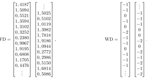
In this situation the household’s fixed demand (FD) and the produced wind energy (WD) over the next 24 hours are known. There are 100 instances used to compare the different strategies. The FD and WD of one instance are given in Figure 4.2. This instance is used to see the dif-ference of the strategies more closely. The values of FD and WD are given as a vector of length 24. Each element of the vector represents respectively the fixed demand and wind demand for the corresponding time. As can be seen from the vectors, the values in the fixed demand vector are positive while the vector for wind energy contains negative values. Wind energy is produced, because supply can be seen as negative demand, the second vector contains negative values.
The wind energy is relatively cheap, when two wind energy units are available, the unit costs will be equal to one, cw2 = 1, when only one unit of wind energy is available the costs for that
unit will be equal to three,cw1= 3. When not enough wind energy is available, energy has to be
FD =
1,4187 1,5094 0,5521 1,3594 1,3102 0,3252 0,2380 0,9967 1,9195 0,6808 1,1705 0,4476
.. . .. . 1,5025 0,5102 1,0119 1,3982 1,7818 1,9186 1,0944 0,2772 0,2986 0,5150 1,6814 0,5086
, WD =
−1 −1 0 −1 0 −2 −1 −1 0 −1 −1 −1 .. . .. . −1 −1 −1 0 0 −2 0 −2 −1 −2 −1 −2 .
Figure 4.2: Fixed demand and wind demand vectors used in the network with known wind pro-duction
WithAw(t) the amount of wind energy used at timetandAf(t) the amount of energy used from flexible energy resources at timet, the total costsT C of the household becomes:
T C =X t
(Aw(t)·cw+Af(t)·cf).
The costs of satisfying all demand in this example network are calculated for each of the strategies, the results are given in Section 6.1.
Wind forecasts
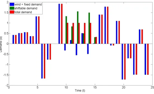
Availability of wind energy in the future can not be known exactly. Wind forecasts are known but change over time. In this part the different strategies are compared to each other when the available information about wind energy changes over time. This comparison is made using 100 instances in the example network given above. The fixed demand vector and wind demand vector of one of these instances are given in Figure 4.3. The fixed demand vector is the same as the fixed demand vector given in Figure 4.2.
FD =
1,4187 1,5094 0,5521 1,3594 1,3102 0,3252 0,2380 0,9967 1,9195 0,6808 1,1705 0,4476
.. . .. . 1,5025 0,5102 1,0119 1,3982 1,7818 1,9186 1,0944 0,2772 0,2986 0,5150 1,6814 0,5086
, WD =
−1,9602
−1,0883
−0,7313
−1,3855
−1,6341
−0,9686
−1,8725
−1,1081
−1,8799
−1,8684
−0,9176
−0,4441 .. . .. .
−1,6782
−1,7621
−1,3225
−1,1182
−0,0668
−1,4268
−1,9537
−1,2481
−0,8068
−1,7736
−1,6504
−0,9810
.
Figure 4.3: Fixed demand and wind demand vectors used in the network with wind forecasts
4. TWO-TIME-SCALE POWERMATCHER
energy resources is relatively expensive, the costs of this kind of energy is set to 10,cf = 10. The wind demand vector will change a little bit at each time t, but stays between zero and minus two. Produced energy can never be positive and can’t exceed the capacity. With n ∈ N and
N ∼ N(0,1):
W Dnew(s) = max( min(W Dold(s) + (0,05·n),0),−2) ∀s≥t.
At timet the vector changes for entriest+ 1, ..., T, entries 1, ..., t−1 do not change because the amount of wind in the past is known for certain. The final wind demand vector (FWD), the wind demand vector at timet= 24 of this instance is given in Figure 4.4.
FWD =
−1,9602
−1,1058
−0,6552
−1,5516
−1,6983
−1,1712
−1,6523
−1,2550
−1,7402
−1,7562
−0,8834
−0,5610 .. . .. .
−1,6365
−1,9942
−0,8771
−0,9787
−0,1510
−1,3234
−2,0000
−1,1069
−0,5251
−1,5955
−1,5263
−1,0626
.
Figure 4.4: Final wind demand vector
The three different strategies will be compared to each other to see how the strategies handle changes in the wind forecasts. The third strategy, where the average price P∗ is assumed to be known, will be divided into two versions. These two versions of the third strategy are now given.
Strategy 3(1)
In this version of strategy 3, the average priceP∗ will only be determined at the first time epoch. The real average price will change in time because of the changed wind demand. The value ofP∗
will not be updated in this strategy.
Strategy 3(24)
In this version of strategy 3, the average price P∗ will be updated at every time epoch. This
strategy thus includes the changes in wind demand.
5
Bidding strategies using Dynamic Programming
The previous chapter, Chapter 4, explained the two-time-scale PowerMatcher and the currently used bidding strategy in the two-time-scale PowerMatcher. Based on this information, new bid-ding strategies can be introduced. The bidbid-ding strategy introduced in this chapter is intended to be used for the shorter time scale and is designed to lead to lower total costs. However, this new bidding strategy could also be used for the larger time scale, in the same way as is explained in this chapter for the shorter time scale.
It is assumed that information about the average price P∗ and the target demand D∗k is al-ready known when the bidding curve for the shorter time scale needs to be calculated, theP∗and
Dk∗are used in the bidding strategy. Some of the other variables that are used in this chapter are listed below.
• p: The variableprepresents the unit price of electricity. The value ofpcan have any value betweenpmin andpmax, the minimum and maximum price.
• ri: The variables ri with i = 1, ..., n give the n possible values ofp that are worked with in the new bidding strategy. Price pis continuous, the bidding strategy introduced in this chapter can only be used when the price is discrete, the variable p therefore needs to be discretized. The values ofri are dependent on the price distribution used.
• qi: The value ofqi shows the probability that the price equalsri. The probabilities are used in the dynamic programming part of the new bidding strategy and the values of qi depend on the price distribution.
• ak(ri;t, d): The value ofak shows the amount of electricity that can best be buyed/sold in the situation with priceri, timetand remaining demand d.
Using the new bidding strategy, the value of ak(ri;t, d) becomes dependent on the remaining demand,d. The form of the bidding curve will therefore be given by:
r1 ak(r1;t, d)
..
. ...
rn ak(rn;t, d)
.
Two steps are needed to determine the bidding curve.
1. The possible values of the price, r1, ..., rn, and the corresponding probabilities q1, ..., qn, are determined.
2. With step 1 completed, theak(ri;t, d) are calculated.
Whenri,qi andak(ri;t, d) are determined for all i, the bidding curve is known.
Section 5.1 shows how the possible values of the price,r1, ...,rn, and the corresponding probabil-ities, q1, ...,qn are determined for the case with known prices and for the case where prices are stochastic. Different levels of information about the prices are used in this second case. With the
ri and qi values known, the values of ak(ri;t, d) can be determined. Section 5.2 shows how the values ofacan be determined when the prices are known. This is done by rewriting the problem as a Knapsack problem and solving this Knapsack problem using dynamic programming. Section 5.3 shows how the values ofacan be determined when the prices are stochastic. Sections 5.2 and 5.3 are explained for the situation where an electric car has to be charged before the end of time
5. BIDDING STRATEGIES USING DYNAMIC PROGRAMMING
5.1
Determine price distribution
The first step in determining the bidding curve is to determine the possible values of the price
p, r1, ..., rn, and the corresponding probabilities, q1, ..., qn for a given value of n. This value of
n determines the number of breakpoints in the bidding curve, where a high value of n means that the demand ak(ri;t, d) is known for more possible values of the price. This leads to more detailed information about the bidding strategy, see Figure 5.1. Different values ofnwill be used throughout the report.
(a) n = 5 (b) n = 25
Figure 5.1: Two examples of a bidding curve
The values ofr1, ...,rnand corresponding probabilitiesq1, ...,qnare in this section determined for different levels of information aboutpt. Section 5.1.1 determinesri when the pricespare known in advance. In sections 5.1.2 till 5.1.4 pt is assumed to be a random variable that can take any of n values, where the value of n is handpicked and assumed to be odd. The n possible values of the price, r1, ..., rn, can be determined using different distributions. The discrete uniform distribution is used in Section 5.1.2, where the average price P∗ is assumed to be known. The normal distribution is used in Section 5.1.3, where besidesP∗also the standard deviation ofp,σp, is assumed to be known. The normal distribution is also used in Section 5.1.4, where the average price and standard deviation at eacht, p∗t andσp,t, are known.
The values ofr1, ...,rn and the corresponding probabilitiesq1, ...,qndetermined in this section are used in Section 5.3, whereak(ri;t, d) is determined for allri,tanddusing dynamic programming.
5.1.1 Knownpt
In this section the prices p1, ...,pT are assumed to be known. With known prices, the number of possible values for the price is equal to one, n = 1. The values ofr1 and q1 thus need to be
determined. The value of r1 at time tshows the only possible value of pt, sor1 =pt. The price
ptis known, thereforeq1= 1. With known prices, the bidding curves have the following form:
pt ak(pt;t, d) Section 5.2 shows how the value ofak(pt;t, d) is determined.
5.1.2 KnownP∗
It is in this section assumed that the pricep is a random variable that can take any of ngiven values, wherenis handpicked and assumed to be an odd number. Thesenpossible values of the price,r1, ...,rn, need to be determined, together with the corresponding probabilities,q1, ..., qn. With the average price P∗ known, the discrete uniform distribution is used to determineri and
the same for eachi,qi=n1 fori= 1, ..., n. The following equation thus holds.
n
X
i=1
qi·ri = P∗.
With stepsizes=pmax−npmin, the resulting bidding curve is specified by:
pmin ak(pmin;t, d)
pmin+s ak(pmin+s;t, d) ..
. ...
P∗ ak(P∗;t, d) ..
. ...
pmax−s ak(pmax−s;t, d)
pmax ak(pmax;t, d)
.
The values of ri andqi are used as inputs for Section 5.3, where ak(ri;t, d) is determined for all
ri,tanddusing dynamic programming.
5.1.3 KnownP∗ and σp
In Section 5.1.2 the values for ri and qi are determined using the discrete uniform distribution, using the average price P∗. In this section it is assumed that the prices are normally distributed with a given average priceP∗ and standard deviation σp, X ∼ N(P∗, σp). This is discretized to a random variablept that can take on any ofngiven values, wheren is again assumed to be an odd number. Now, the values of ri andqi, fori= 1, ..., nhave to be determined such that these values correspond to the given normal distribution.
As the interval [P∗−3σp, P∗ + 3σp] covers 99,7 % and thus “almost all” of the range of x, the valuesri fori= 1, ..., nare all chosen in the interval [P∗−3σp, P∗+ 3σp], more precisely they are determined as follows: First, the interval [P∗−3σp, P∗+ 3σp] is decomposed inton equally sized intervals. Figure 5.2 shows these intervals forn=5.
Figure 5.2: Intervals whenn=5
Withxi=P∗−(3−n6·i)σp, intervaliis denoted by [xi−1, xi]. Next, the area left of P∗−3σpis added to the first interval and the area right ofP∗+ 3σpis added to then’th interval, sox0=−∞ andxn =∞. Then, for alli, the valueri is calculated in such a way that ri is the average price of intervali. At interval n+12 the curve is symmetric aroundP∗, so:
rn+1 2
5. BIDDING STRATEGIES USING DYNAMIC PROGRAMMING
The values ri for alli6= n+12 are more difficult to determine, because the curve is not symmetric in these intervals. At intervali with bounds [xi−1, xi], ri is the expected value ofxgiven thatx is in interval [xi−1, xi].
ri=E[x|x∈[xi−1, xi]].
The valueri is such that:
P(xi−1<X<ri) =
1
2P(xi−1<X<xi). (5.1.1) The normal distribution probabilities can be calculated through the standard normal distribution.
P(xi−1<X<xi) ≈ Φ
x
i−P∗
σp
−Φ
x
i−1−P∗ σp
.
Now that the values ofri,i= 1, ..., nare known, the values ofqi,i= 1, ..., nhave to be calculated. The valueqi corresponding tori is the probability to be in intervali.
qi ≈ Φ
x
i−P∗
σp
−Φ
x
i−1−P∗ σp
. (5.1.2)
When the values ofri andqi are known fori= 1, ..., n, the bidding curve:
r1 ak(r1;t, d)
..
. ...
P∗ ak(P∗;t, d) ..
. ...
rn ak(rn;t, d)
can be determined using dynamic programming, explained in Section 5.3.
5.1.4 Knownp∗t and σp,t
In this section the values ri and qi for i= 1, ..., nare again determined using the normal distri-bution. Where in the previous section the valuesri and qi were determined using P∗ andσp, in this section the valuesri andqi are determined for eacht seperately using information about the average price and standard deviation at that specific time, denoted by p∗t andσp,t. The average price p∗t is thus the average price at only time t, where P∗ at time t represents the expected average price from timetuntilT. The same holds forσp,tandσp. The price at timetis normally distributed, at each timet letX ∼ N(p∗t, σp,t). Then for eacht, this is discretized to a random variable pt, as explained in Section 5.1.3. Based on the values p∗t and σp,t, n intervals are made and the valueri in each interval [xi−1, xi] fori= 1, ..., nis determined such that Equation (5.1.1)
holds. The values ofqi, for alli= 1, ..., n, are determined using Equation (5.1.2). These values of
ri andqi are determined for each tseperately. The values of ri andqi can be different for eacht. These values are therefore denoted byri,t andqi,t. The bidding curve attis now given by
r1,t ak(r1,t;t, d) ..
. ...
p∗t ak(p∗t;t, d) ..
. ...
rn,t ak(rn;t, d)
5.2
DP using known prices
This section shows how to find ak(ri;t, d) for allri,t anddwhen all pricesp1, ...,pT are known. Note thatn= 1 whenptis known, the values ofak(p1;t, d), ..., ak(pT;t, d) need to be calculated. The problem of calculating these values can be rewritten as a Knapsack problem, see [19], and this Knapsack problem can be solved using dynamic programming.
The problem of finding ak(p1;t, d), ..., ak(pT;t, d) is first transformed to the Knapsack prob-lem.
There is a number of time epochst= 1, ..., T and each time has a corresponding pricept. A total ofW units of shiftable demand need to be satisfied at the end of timet and only a maximum of
mtunits of demand can be satisfied at timet. The decision variablext is the amount of demand satisfied at timet. The problem is to minimize the total costs of satisfyingW units of demand.
minimize T
X
t=1
pt·at (5.2.1)
subject to T
X
t=1
at≥W,
xt∈ {0,1, ..., mt}, t= 1, ..., T.
This Knapsack problem can be solved using dynamic programming.
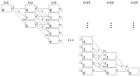
How the problem is solved by dynamic programming is shown using a numerical example. In this exampleT = 24,W = 8,mt= 2 andptfort= 1, ...,T is shown in the vector below.
p =
5 5 4 4 3 4 4 5 5 6 6 6 . . .
. . . 5 4 4 5 5 6 6 7 6 5 5 4
.
Now a decision tree can be made. The tree corresponding to the numerical example is given in Figure 5.3. The nodes in the tree are of the form (t, d), where t specifies the time and d the remaining demand.
Figure 5.3: Tree withT= 24,W = 8 andmt= 2
5. BIDDING STRATEGIES USING DYNAMIC PROGRAMMING
of an edge represents the costs at timetwhenatis satisfied att.
e((t, d),(t+ 1, d−at)) = pt·at ∀t, d, a.
Each path in the tree from node (t, d) to (T + 1,0) now corresponds to a feasible solution for satisfying demanddin time epochst, ...,T.
For solving problem (5.2.1) the minimum costs from node (t, d) to node (T + 1,0) is needed for eacht andd, the minimum costs from node (t, d) to node (T+ 1,0) is also called the value of node (t, d), denoted byVt(d). Especially, the value of node (1, W) is interesting. TheV1(W) shows the minimum costs for satisfying all demand over all times. Also, the minimum costs path from node (1, W) to node (T+ 1,0) shows the best action at eacht. BeforeV1(W) can be determined,
theVt(d) need to be determined for allt>1, starting withVT+1(d). The value of nodes (T+ 1, d)
for alldare given in equations 5.2.2 and 5.2.3. At time T+ 1 the remaining demanddneeds to be exactly zero,VT+1(d) is therefore equal to zero when d= 0 and set to infinity when the node
is not reachable, i.e.,d6= 0.
VT+1(d) = 0 d= 0, (5.2.2) VT+1(d) = ∞ d6= 0. (5.2.3)
For all othert, the value of node (t, d) is given by equation 5.2.4. InVt(d), pt·at is the costs for usingatat tandVt+1(d−at) is the costs for usingd−atfrom t+ 1 toT.
Vt(d) = minat[pt·at+Vt+1(d−at)] t=T, ...,1. (5.2.4)
Working backwards fromT to 1,Vt(d) and correspondingatcan be determined for all nodes (t, d), including the desired V1(W). At timeT all remaining demand dneeds to be satisfied. There is
therefore only one action: satisfy alld. The values of the nodes at time t= 24 in the numerical example are given below. Becausemt= 2, the nodes (24,8), ..., (24,3) can not reach (25,0) and the values of these nodes are therefore set to infinity.
V24(8) = ∞,
.. . ...
V24(3) = ∞,
V24(2) = p24·2 +V25(0)
= 8,
V24(1) = p24·1 +V25(0) = 4,
V24(0) = p24·0 +V25(0) = 0.
At timet≤T−1 there are more choices. The values of nodesV23(8), ...,V23(0) in the numerical
example are given next.
V23(8) = ∞,
.. . ...
V23(5) = ∞,
V23(3) = min[p23·2 +V24(1), p23·1 +V24(2)] = min[10 + 4,5 + 8] = 13,
V23(2) = min[p23·2 +V24(0), p23·1 +V24(1), p23·0 +V24(2)]
= min[10 + 0,5 + 4,0 + 8] = 8, V23(1) = min[p23·1 +V24(0), p23·0 +V24(1)]
= min[5 + 0,0 + 4] = 4, V23(0) = p23·0 +v24(0)
= 0 + 0 = 0.
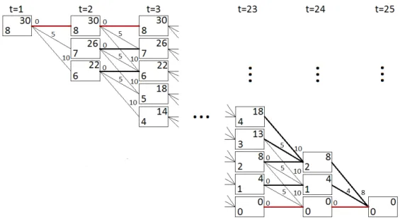
The values of all other nodes are determined in the same way. The values of the nodes are given in the upper right corner of the nodes in Figure 5.4. It is assumed that if the value of a certain node is obtained by multipleatthe highest value ofatis chosen. The edge (value of at) to choose at each of the nodes is shown in the figure as a wider edge. The wider edge is coloured red when the edge is part of the minimum costs path from node (1, W) to node (T+ 1,0), the path that is most interesting.
Figure 5.4: Node values and best actions withT = 24,W = 8 andmt= 2
Now, at t = 1 the value of at is known for each t. With these values of at known, the bid-ding curve can already be made for eacht. The bidding curve at timet with remaining demand
dis given by:
pt ak(pt;t, d).
Finding the value of at and the bidding curve at time t becomes more difficult when the prices are forecasted instead of known. Section 5.3 shows how these values are determined when price distributions are used.
5.3
DP using price distributions
5. BIDDING STRATEGIES USING DYNAMIC PROGRAMMING
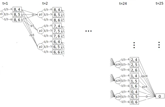
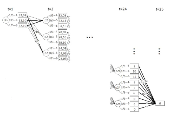
fori= 1,2,3. With this information a decision tree can be made. The tree corresponding to the given example is given in Figure 5.5. This tree consists of two kinds of nodes and has therefore a different form than the tree given in Figure 5.3. At eacht, firstptis determined, this is done at the chance node (shown in the figure as a circle). Theptcan take on valuesr1, ...,rn. Withptknown, the decision about the value of at can be made, this is done at the decision node (rectangular node). The rectangular nodes are of the form (t, d) and show the current state, [d, pt]. Edges from a chance node to a decision node show the value ofri and the probability qi of ri. The weight of the edges from decision nodes to chance nodes represent the costs at timet, whenatis satisfied.
Figure 5.5: Tree withT= 24,W = 8 andmt= 2
Each path in the tree now corresponds to a feasible solution for satisfying demand din times t, ...,T.
The total costs need to be minimized, equations 5.2.2 till 5.2.4 can’t be used for this, thept+1,
...,pT are unknown at timet and thereforeVt+1(d−at) is also unknown. The price distribution however is known and therefore the expected values of the nodes can be calculated. The expected value of node (t, d),EVt(d), shows the expected minimum costs for satisfyingdat timest+ 1, ...,
T with a given price distribution. At timeT+ 1 the remaining demanddneeds to be exactly zero,
EVT+1(d) is therefore equal to zero whend= 0 and set to infinity when the node is not reachable,
i.e.,d6= 0.
EVT+1(d) = 0 d= 0, (5.3.1) EVT+1(d) = ∞ d6= 0. (5.3.2)
For all othert, the expected value of node (t, d) is given by equation 5.3.3. InEVt(d),ri·atis the costs for usingatat twith priceri,EVt+1(d−at) gives the expected costs for usingd−atfrom timet+ 1 toT.
EVt(d) = X i
qiminat [ri·at+EVt+1(d−at)] t=T, ...,1. (5.3.3)