University of Warwick institutional repository: http://go.warwick.ac.uk/wrap This paper is made available online in accordance with
publisher policies. Please scroll down to view the document itself. Please refer to the repository record for this item and our policy information available from the repository home page for further information.
To see the final version of this paper please visit the publisher’s website. Access to the published version may require a subscription.
Author(s): Neil Stewart
Article Title: Millisecond accuracy video display using OpenGL under Linux
Year of publication: 2006
Link to published version: http://brm.psychonomic-journals.org/content/38/1/142.full.pdf+html
Running Head: LINUX VIDEO DISPLAY
Millisecond Accuracy Video Display Using OpenGL Under Linux
Neil Stewart
University of Warwick, England
Stewart, N. (2006). Millisecond accuracy video display using OpenGL under Linux. Behavior
Research Methods, 38, 142-145.
Neil Stewart
Department of Psychology
University of Warwick
Coventry
CV4 7AL
England
+44 24 7657 3127
Abstract
To measure people's reaction times to the nearest millisecond, it is necessary to know exactly
when a stimulus is displayed. This article describes how to display stimuli with millisecond
accuracy on a normal CRT monitor using a PC running Linux. A simple C program is
presented to illustrate how this may be done within X Windows using the OpenGL rendering
system. A test of this system is reported that demonstrates that stimuli may be consistently
displayed with millisecond accuracy. An algorithm is presented that allows the exact time of
stimulus presentation to be deduced, even if there are relatively large errors in measuring the
Millisecond Accuracy Video Display Using OpenGL Under Linux
In many psychology experiments, a stimulus is presented and the latency of a
participant's response is recorded. There are two key pieces of information that are required to
determine a participant's reaction time: the time that the stimulus was presented and the time
that the participant responded. I describe how to record responses with millisecond accuracy
under Linux in Stewart (2004). This article is concerned with presenting stimuli with
millisecond accuracy.
A Choice of Display Method
A standard cathode ray tube (CRT) monitor works by scanning a beam of electrons
over a phosphorus-coated screen. When the beam strikes the phosphorus, the phosphorus
fluoresces. The beam scans each row of pixels from left to right, beginning with the top row
and ending with the bottom row. The intensity of the beam is varied with location, to cause
the phosphorus to fluoresce with different intensity, allowing a picture to be built up over a
scan of the whole screen. The number of scans of the entire screen per second is called the
refresh rate.
Recently, liquid crystal displays (LCDs) have been introduced. These work quite
differently. When a voltage is applied to a liquid crystal, it changes its shape. Different shaped
crystals rotate the plane of polarized light by different extents. In an LCD, a layer of liquid
crystals is sandwiched between two orthogonal polariods. Unless the plane of the polarized
light is rotated in between the two polariods it cannot pass through them. By varying the
voltage applied to the liquid crystals in the sandwich, the degree of rotation of the plane of the
polarized light varies, allowing more or less light to pass through the LCD. By having a large
array of liquid crystal segments, each controlled independently, the amount of light passing
through different parts of the LCD can be controlled to create a picture. In thin film transistor
(TFT) LCD panels, a transistor and capacitor assembly for each pixel is used to maintain the
Plant, Hammond, and Turner (2004) studied the performance of some CRT displays
and some TFT LCD displays, by measuring the time for the display to become visible (as
measured by a photodiode and oscilloscope apparatus). The CRTs tested reached full
brightness in less than 1 ms. However, the brightness of the LCDs tested changed very
slowly, taking 10 - 20 ms for the display to reach full brightness (i.e., to warm up), depending
on the display. Further, the LCD displays took 5 - 20 ms for the image to fade to the
background level of brightness on stimulus offset (i.e., to cool down).1 The point during the
warm-up time at which an image is detectable by a human observer and similarly the point
when it is no longer visible during the cool-down time is likely to vary with environmental
factors (e.g., ambient illumination, the brightness of other stimuli) and history (e.g., the
brightness of recent stimuli). Thus, Plant et al.'s study shows that LCD TFT displays are not
suitable for presenting stimuli with millisecond accuracy. Here I describe how to control a
CRT display with millisecond accuracy in Linux.
A Simple Linux Program2
The most commonly used graphics system under Linux is X Windows. X Windows
provides a graphical engine that is hardware independent and used across a large variety of
operating systems such as Mac OS X and Sun Solaris. Linux systems usually use a free
implementation of the X Windows standard called XFree86 (http://www.xfree86.org/). The X
Windows system performs windowing tasks, such as allocating new windows, moving them
around, and deciding when they need to be redrawn. In this simple program I have used the
OpenGL graphics library to draw into a new window that fills the entire screen. OpenGL is
also hardware independent and runs on many other operating systems. I used the Mesa3D
implementation of the OpenGL standard (http://www.mesa3d.org/).3
The complete C source code for the program is available from
http://www.warwick.ac.uk/staff/Neil.Stewart/. The program first creates a blank, borderless
would like more information than is provided by the man pages for these functions, consult
Nye (1992) and Woo, Neider, Davis, & Shreiner (1999). First, XOpenDisplay is used to open
a connection to the X Server and obtain server display information. Second, glXChooseVisual
is used to select, from all available visuals on the display, the type of visual that best meets a
minimum specification. Third, glXCreateContext is used to create a rendering context with
direct access to the video card. Fourth, a new window that fills the entire screen and has no
border is made using XCreateWindow. The attributes for this window are extracted from
those of the root window. Fifth, to display or map the window to the screen XMapWindow is
called followed by XIfEvent. XIfEvent waits for the window to be displayed before allowing
execution to proceed.
So far, a new window has been created with an OpenGL rendering context that
renders directly to the video card. Next, the details of the OpenGL system need to be
specified. The rendering context is selected with glXMakeCurrent, and the coordinate system
established with glViewport. OpenGL, which is a 3D rendering system, can be set to 2D by
setting the model and projection transforms to the identity matrix (by calling glMatrixMode
and glLoadIdentity) and calling glOrtho2D.
The final step is to hide the cursor. Unfortunately, to hide the cursor X Windows
requires the creation of a blank cursor using XCreatePixmapCursor by passing a blank pixmap
created with XCreateBitmapFromData as a parameter. The cursor is defined as the current
cursor using XDefineCursor. Together, all of these steps may seem rather lengthy, but they
will work on any X Windows System with OpenGL.
From this point, things are much more simple. The rendering context that the program
selects is a double buffered context. In double buffering, while the contents of one buffer are
being displayed, drawing takes place on the other buffer. When a glXSwapBuffers call is
made, the roles of the two buffers are reversed.The reversal is synchronized to the screen
corner at the end of a trace back to the top left corner for the beginning of the next. This
means that, if buffers are swapped every frame, there is one frame period (e.g., 10 ms at 100
Hz refresh rate) for drawing into a buffer. Because modern computers are are very fast, it is
possible to draw an awful lot in this time (cf. current computer games like Doom 3 and
Half-Life 2) depending on the processor and graphics card. There is no longer a need to buffer a
really large number of frames in advance (cf. only 5 years ago, Graves & Bradley, 1988a,
1988b; Myors, 1998, 1999; Tsai, 2001).
As an example, the following code fragment draws a red rectangle in the center of a
green screen.
glClearColor(0.0, 1.0, 0.0, 1.0);
glClear(GL_COLOR_BUFFER_BIT);
glColor3f(1.0,0.0,0.0);
glRecti(-100,-100,100,100);
glXSwapBuffers(display, window);
glFinish();
gettimeofday(time, (struct timezone *) 0);
The clear color is set with glClearColor (which takes red, green, blue, and alpha values) before
the screen is cleared by glClear. The drawing color is set to red by glColor3f (which takes red,
green, and blue values) and a rectangle is drawn with glRecti with the bottom left corner at
-100, -100 and the top right corner at 100, 100. The call to glXSwapBuffers swaps the
buffers, displaying the rectangle. The glFinish call ensures that all commands are complete
before it returns. Thus the call to gettimeofday sets the variable time to the time at which the
tracing of first frame containing the rectangle began.
A Test of Millisecond Accuracy
I conducted a simple test of the accuracy of the times recorded as above. I set up a
white, and recorded the time after every call to glXSwapBuffers and glFinish. If the times are
accurate, then the intervals between times should be exactly the refresh period.
The system I ran these tests on is a dual processor 1.4 MHz AMD Athlon with 256
MB of RAM with a PCI NVidia GeForce 2 MX with 32 MB of video RAM. I used the
Debian Woody GNU distribution with a 2.4.25-1-k7-smp Linux kernel, XFree86 4.1.0 and the
NVidia 1.0-5336 driver4 (and not the nv driver that comes with XFree86). The CRT monitor
was a Sony CPD-G220 Color Trinitron running with a refresh rate of 85 Hz. The following
source code was used to sample the time of 10,000 consecutive refreshes.
for(i=0; i<10000; i++) {
c=double(i%2);
glClearColor(c, c, c, 1.0);
glClear(GL_COLOR_BUFFER_BIT);
glXSwapBuffers(display, window);
glFinish();
gettimeofday(time[i], (struct timezone *) 0);
}
By alternating the color of the screen on alternate refreshes between black and white (using
the variable c), a photodiode apparatus that was connected to the screen could detect the
refreshes. During the test, no refreshes were missed (i.e., the screen color swapped every 1/85
s).
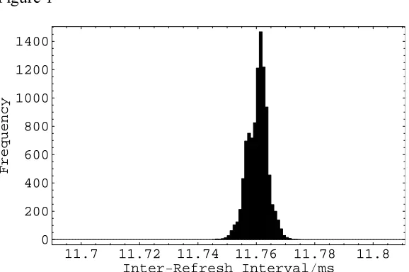
For a vertical refresh rate of 85 Hz, the period should be 11.765 ms. Figure 1 shows
the differences between the consecutive times recorded in the array time. Only 12 intervals
(about 1 in 1000) fell outside that range ± 0.05 ms from the expected value of 11.765 ms.
These cases occurred on the six occasions when there was a large gap between the calls to
glXSwapBuffers and glFinish and the call to gettimeofday. The large gap caused the preceding
underestimated by the same amount. The largest error was 5 ms. The very rare errors of up to
5 ms may not be of any concern, because they are so rare, but if they are, fortunately, they are
very easy to correct using the algorithm described below.
A second, more realistic test was also run. The duration of a white screen presented
for 1000 ms (i.e., 85 retraces at an 85 Hz refresh rate) was measured for each of 1000 trials.
The inter-trial interval was also 1000 ms, during which time a black screen was presented. The
total duration of the test was about half an hour. Across the 1000, trials the minimum recorded
display time was 999.734 ms and the maximum was 999.800 ms. This gives a total range of
only 0.066 ms for the stimulus durations, which is an accuracy of better than one tenth of a
ms.5
A Simple Correction
For a monitor driven at v Hz, the times of the beginnings of the refresh must all be 1 /
v s apart. By taking advantage of this fact, the exact time of stimulus retraces can be deduced,
providing the error in recording them is small compared to the refresh period 1 / v. This model
can be formalized in Equation 1.
ti = t0 + i / v (1)
where ti is the time (in s) of the ith retrace and i indexes the number of retraces since the first
at time t0. Suppose that one has recorded a series of retrace times rj (where j indexes the
number of recordings since t0) and that there is some noise in the recording that varies from
trial to trial, so that
rj = ti + j (2)
where j > 0 is the error in recording the time. From Equations 1 and 2, rj - t0 = i / v + j. In
other words, apart from the error in recording the time, rj - t0 must be an integer multiple of
the refresh period 1 / v. Under the assumption that j < 1 / v, then
i = Quotient[rj - t0 , 1 / v ] (3)
by the second. That is, the retrace i on which the jth recording rj was made can be determined.
Once i is known, the exact time of the retrace i is given by Equation 1.
t0 is, however, not known exactly. But it can be estimated from the data. First,
construct the error term
error = (Mod[rj - t0, 1 / v])2 (4)
where the function Mod[ . , . ] returns the remainder after the first parameter is divided by the
second. Error is the squared deviation between the recorded time rj and the first preceding
modeled retrace time (the location of which is determined by t0). Second, average this term
over all of the refresh times recorded. Third, find the value of t0 for which this sum is a
minimum.
To test this algorithm, I have generated 1000 trials of artificial refresh data using
Equations 1 and 2 as follows. The retraces on which recordings were made (i.e., the is) were
generated by starting with a seed value of i = 0, and generating each subsequent value by
adding to the previous value an integer drawn at random from a uniform distribution of
integers between 1 and 20. In this way, the retraces recorded were irregularly spaced, as they
might be in an experiment where the inter-stimulus intervals depend on a participant's response
times. The noise j was modeled as a log normal distribution with mean 2 ms and standard
deviation 2 ms. This standard deviation is 20 times greater than the variability observed in the
above practical test, and so this test is comparatively very tough. t0 was set to an arbitrary
value of 325 ms. In this way, 1000 simulated rjs were generated.
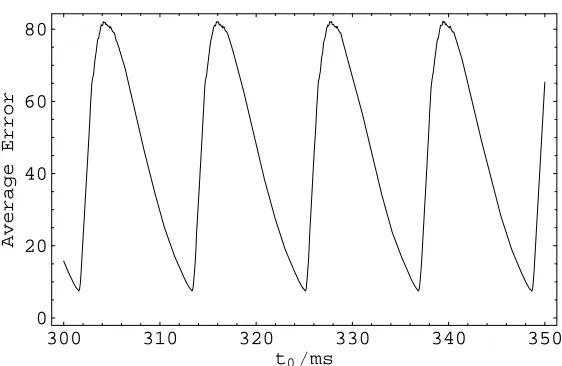
The average error (Equation 4) is plotted as a function of t0 in Figure 2. The function is
periodic, and has a minimum every 1 / v s. The minima immediately preceding r0 is t0. Once t0
is known, Equation 3 can be used to recover the numbers of the retraces (i.e., the is) upon
which the recordings were made. Substituting these is into Equation 1 allows the exact retrace
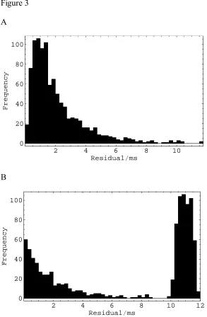
times to be calculated. As a check, the distribution of residuals (rj - ti) can be plotted. Figure
distribution becomes bimodal. Figure 3B illustrates this occurring when t0 = 315.
In summary, by taking advantage of the fact that retraces can only occur at certain
predefined times, noisy timing data can be cleaned up, providing a much better estimate of the
time at which a stimulus is displayed and eliminating trial-to-trial variability. Although the
Linux system described above almost always performed very accurately, this method allows
the very rare errors to be corrected.
Conclusion
In conclusion, a PC Linux system and a CRT monitor can be used to display stimuli
References
Graves , R., & Bradley, R. (1988a). More on millisecond timing and tachistoscope
applications for the IBM PC. Behavior Research Methods, Instruments, & Computers,
20, 408-412.
Graves, R., & Bradley, R. (1988b). Millisecond timing on the IBM PC/XT/AT and PS/2: A
review of the options and correction for the Graves and Bradley algorithm. Behavior
Research Methods, Instruments, & Computers, 23, 377-379.
Finney, S. A. (2001). Real-time data collection in Linux: A case study. Behavior Research
Methods, Instruments, and Computers, 33, 167-173.
MacInnes, W. J., & Taylor, T. L. (2001). Millisecond timing on PCs and Macs. Behavior
Research Methods, Instruments, & Computers, 33, 174-178.
Myors, B. (1998a). The PC tachistoscope has 32 pages. Behavior Research Methods,
Instruments, & Computers, 30, 457-461.
Myors, B. (1999). The PC tachistoscope has 240 pages. Behavior Research Methods,
Instruments, & Computers, 31, 329-333.
Nye, A. (1992). Xlib programming manual (3rd ed.). Sebastopol, CA: O'Reilly.
Plant, R. P., Hammond, N., & Turner, G. (2004). Self-validating presentation and response
timing in cognitive paradigms: How and why. Behavior, Research Methods,
Instruments, & Computers, 36, 291-303.
Stewart, N. (2004). A PC parallel port button box provides millisecond response time
accuracy under Linux. Manuscript submitted for publication.
Tsai, J. L. (2001). A multichannel PC tachistoscope with high resolution and fast display
change capability. Behavioral Research Methods, Instruments, & Computers, 33,
524-531.
Woo, M., Neider, J., Davis, T., & Shreiner, D. (1999). OpenGL programming guide (3rd
Author Note
Neil Stewart, Department of Psychology University of Warwick.
I thank Dave Sleight for constructing the photodiode apparatus and James Adelman
and Matthew Roberts for sharing their Linux knowledge.
Correspondence concerning this article should be addressed to Neil Stewart,
Department of Psychology, University of Warwick, Coventry, CV4 7AL, UK. E-mail:
Footnotes
1Plant et al. (2003) also found that there was a delay of up to 50 ms between the time
that E-prime software was scheduled to display the image and the time the image began to
appear on the display.
2For a multitasking operating system (e.g., Linux, MacOS X, or MS Windows) to be
able to function with millisecond accuracy, one must prevent the program from being
interrupted and having its memory swapped to disc. An accurate timer is also required. Finney
(2001; see also MacInnes & Taylor, 2001; Stewart, 2004) describes how to ensure a Linux
program meets this standard.
3The OpenGL utility toolkit (GLUT) can be used to simplify the process of initializing
and opening new windows and controlling window events. In GLUT, buffers are swapped by
calling glutSwapBuffers, which in turn calls glXSwapBuffers.
4To ensure that buffers are swapped only during the vertical blanking period by
glXSwapBuffers, the environment variable __GL_SYNC_TO_VBLANK must be set to a
non-zero value. It is easy to spot when buffer swapping is not synchronized, because the
screen seems to "tear".
5The fact that the total display time was slightly less than 1000 ms indicates either that
the actual monitor refresh rate was slightly faster than 85 Hz or that the computer's clock is
running slightly slow. The clock on the test computer loses about 2.6 x 10⁻⁷ s per s, as
Figure Caption
Figure 1. The distribution of inter-refresh intervals measured by a gettimeofday call after a
glXSwapBuffers and a glFinish.
Figure 2. Model error as a function of t0.
Figure 1
11.7 11.72 11.74 11.76 11.78 11.8 Inter-Refresh Intervalms
0 200 400 600 800 1000 1200 1400
Figure 2
300 310 320 330 340 350
t0ms 0
20 40 60 80
Average
Figure 3
A
2 4 6 8 10
Residualms 0
20 40 60 80 100
Frequency
B
2 4 6 8 10 12
Residualms 0
20 40 60 80 100
![138 Phishing [ PUNISHER ] pdf](data:image/gif;base64,R0lGODlhAQABAIAAAP///wAAACH5BAEAAAAALAAAAAABAAEAAAICRAEAOw==)