Fiber depolymerization

University of Warwick institutional repository: http://go.warwick.ac.uk/wrap

This paper is made available online in accordance with

publisher policies. Please scroll down to view the document

itself. Please refer to the repository record for this item and our

policy information available from the repository home page for

further information.

To see the final version of this paper please visit the publisher’s website.

Access to the published version may require a subscription.

Author(s): M.S. Turner, G. Agarwal, C.W. Jones, J.C. Wang, S. Kwong,

F.A. Ferrone, R. Josephs and R.W. Briehl

Article Title: Fiber Depolymerization

Year of publication: 2006

Link to published version:

Fiber Depolymerization

M. S. Turner,* G. Agarwal,

C. W. Jones,* J. C. Wang,

S. Kwong,

F. A. Ferrone,

R. Josephs,

and R. W. Briehl

*Department of Physics, University of Warwick, Coventry, United Kingdom;yDepartment of Physiology & Biophysics, Albert Einstein College of Medicine, Bronx, New York;zDepartment of Physics, Drexel University, Philadelphia, Pennsylvania; and§_{Department of Molecular Genetics & Cell Biology, University of Chicago, Chicago, Illinois}

ABSTRACT

Depolymerization is, by definition, a crucial process in the reversible assembly of various biopolymers. It may

also be an important factor in the pathology of sickle cell disease. If sickle hemoglobin fibers fail to depolymerize fully during

passage through the lungs then they will reintroduce aggregates into the systemic circulation and eliminate or shorten the

protective delay (nucleation) time for the subsequent growth of fibers. We study how depolymerization depends on the rates of

end- and side-depolymerization,

k

and

k

, which are, respectively, the rates at which fiber length is lost at each end and the

rate at which new breaks appear per unit fiber length. We present both an analytic mean field theory and supporting simulations

showing that the characteristic fiber depolymerization time

t

¼

1

=

p

ffiffiffiffiffiffiffiffiffiffiffiffiffiffiffiffiffiffi

kendkside

depends on both rates, but not on the fiber length

L

,

in a large intermediate regime 1

k

L

2

/

k

(

L

/

d

)

, with

d

the fiber diameter. We present new experimental data which

confirms that both mechanisms are important and shows how the rate of side depolymerization depends strongly on the

concentration of CO, acting as a proxy for oxygen. Our theory remains rather general and could be applied to the

depoly-merization of an entire class of linear aggregates, not just sickle hemoglobin fibers.

INTRODUCTION

The assembly of particular proteins, or other monomers, into

long polymeric fibers is of great importance in the function

of the living cell as well as chemistry in general. This

poly-merization process can often be reversible, as in actin filaments

or microtubules (1) or living polymers, such as wormlike

surfactant micelles (2). Whereas the phenomenon of

poly-merization has been studied in great detail, that of

depoly-merization has received rather less attention. This is despite

the fact that depolymerization processes are now believed to

play an important role in sickle cell disease and may even be

relevant in amyloid-based diseases if they affect the

persis-tence of fibrils.

We believe that the theoretical analysis that we present in

this article could have rather wide application in

understand-ing depolymerization processes in general. However, this

study was initially motivated by experiments that

demon-strated the feasibility of measuring the depolymerization of

individual sickle cell fibers (3). New quantitative data is now

available that is suitable for comparison with our theory, as

we will report below. We hope that the connection that our

model makes with microscopic kinetic rates may motivate

future experiments on depolymerization of other polymers,

perhaps including amyloid fibrils.

Sickle hemoglobin fibers are sometimes formed by mutant

hemoglobins (HbS), e.g., when they are deprived of oxygen.

These fibers rigidify red blood cells and are a primary,

ini-tiating cause of sickle cell disease (4). It is important to

understand the kinetics that control both the polymerization

and depolymerization of these fibers as both of these

pro-cesses are important in controlling the effects of the disease.

We will consider only depolymerization in the remainder of

this article.

The association kinetics of sickle hemoglobin fibers have

been well characterized and have been shown to be described

by the double-nucleation model of Ferrone et al. (5,6). In this

model the initial nucleation of fibers is homogeneous and

highly cooperative with a rate that is a high power of the

pro-tein concentration. Subsequently, new fibers are also formed by

heterogeneous nucleation on the surfaces of existing fibers,

so that the rate of new fiber formation is proportional to the

mass of fiber already present, leading to exponential kinetics.

All fibers grow by addition of monomers at fiber ends.

In sickle cell disease, polymers form under deoxygenating

conditions and depolymerize if the oxygen concentration is

high. If depolymerization is slow, sickle fibers may fail to

dissolve during their passage through the oxygenating

con-ditions provided by the lungs, typically lasting 1–3 s (7). As

we will discuss below, slow depolymerization may often be

associated with conditions in which the fibers depolymerize

by loss of materials from their ends (only), a process which

we will refer to as end-depolymerization. If

depolymeriza-tion is slow, residual polymers may pass into the systemic

cir-culation, eliminate the protective nucleation-dependent delay

time, and thus may predispose the patient to acute sickle cell

crises. As we will discuss below, an additional mode of

depolymerization, which we will refer to as

side-depoly-merization, is also possible and can greatly decrease the time

required for fibers to fully depolymerize. The side-end

depolymerization mechanism, which involves loss of

mate-rial from fiber midsections, may apply to other biological

Submitted September 29, 2005, and accepted for publication May 4, 2006. Address reprint requests to Dr. Matthew S. Turner, Tel.: 44-24-7652-2257; E-mail: [email protected].

polymers and may thus have bearing on normal physiology

as well as pathophysiology. We therefore suggest that the

results of our theoretical analysis may be relevant to

scientists who are interested in polymer kinetics in general.

Recent experiments by Agarwal et al. (3) clearly show that

sickle hemoglobin fibers can depolymerize both by loss of

monomers from the fiber ends and by side

depolymeriza-tion, which involves loss of material from midsections of

the fiber. Electron micrographs of partially depolymerized

fibers presented in this earlier study seem to suggest that

side-depolymerization may correspond to the formation of

breaks in the fiber. The fiber may not always break as cleanly

as these micrographs suggest, but may leave ends that

resemble, e.g., sharpened sticks. This is natural, given that

sickle hemoglobin fibers are made up of a twisted bundle of

seven double strands of HbS and those proteins residing in

the outermost strands may leave before those in the inner

strands. However, provided the length of any resulting

ta-pered section near the end remains small compared to the

average length of the fiber fragments, we can neglect such

details, treating the polymer as a quasi-one-dimensional

ob-ject in what follows. Finally, it may be worth noting that

end-depolymerization appears to occur at the same rate at both

(all) ends of the fiber.

The new pairs of ends that result from the formation of such

breaks in the fiber would then provide new sites for the loss of

material via end-depolymerization. Clearly, if there are many

such breaking events during the course of the

depolymeriza-tion of a typical fiber, then the kinetics will depend crucially

on both the rates of end- and side-depolymerization (3). In this

article, we aim to provide a quantitative analysis of this effect.

Clearly, similar depolymerization mechanisms may be

im-portant in other fibrillar protein aggregates.

It is worth noting that, in a sense, our depolymerization

model mirrors that of polymerization: For depolymerization,

there is nucleation of holes, whereas in polymerization, there

is the nucleation of aggregates. We study depolymerization

(alone) in this article by restricting our attention to

thermo-dynamic (chemical) conditions in which net association is

negligible, as can be easily achieved for sickle hemoglobin

and other so-called living polymers.

THEORY

We consider a fiber of lengthLthat, at timet¼0, starts to depolymerize via two mechanisms: 1), end-depolymerization at ratekendin units ofmm s1;

and 2), side-depolymerization, described by the formation of breaks (new pairs of ends) at random positions with a rateksidein units ofmm

1

s1(see Fig. 1). This second process is assumed to involve the formation of holes of constant initial sized, equivalently the loss of a segment of fiber of lengthd. Once created, the holes then grow via end depolymerization of the newly created end pairs. A complete mathematical treatment must deal not only with the creation of ends but also their annihilation, which occurs whenever any small segment of fiber vanishes by shrinkage of its ends to a point. Such events may occur frequently for fibers that have significant side-depoly-merization rates, as we will show below.

The kinetics of the depolymerization process that result from this model are as follows: For fibers that are subject to a very slow breaking rate, fiber shrinkage occurs via depolymerization at its two original ends (only), leading to fiber disappearance on the timescale

t

¼

L

=

ð

2kend

Þ

:

(1)

This has been observed (3) to occur with a ratekend0.5mm s1. As the

breaking (side-depolymerization) rateksideincreases, controlled by, e.g., an

increase in oxygen (or CO) concentration, the appearance of breaks remains rare on average, until the dimensionless parameterxgiven by

x

[

k

L

₌

k

(2)

reachesx*1. At this point, the average maximum number of extra ends formed in timetend, given bynmax’ksideLtend’x, exceeds unity and thus

hole formation cannot be neglected whenx*1. The characteristic timescale on which the fiber disappears then remains well approximated by

t

¼

1

=

p

ffiffiffiffiffiffiffiffiffiffiffiffiffiffi

kendkside

;

(3)

provided 1x(L/d)2, withdthe initial size of holes, probably of the order of the fiber thickness. We will fully justify this result, and its regime of validity, in what follows. This timescale has the striking feature that it does not depend on the initial fiber lengthL. Finally, the side-depolymerization rate may becomes so large that the entire fiber disappears rapidly by simul-taneous side-depolymerization of all its segments on the timescale

t

¼

1

=

ð

k

d

Þ

:

(4)

This is the fastest mechanism whentsidet, which only occurs when x(L/d)2, thereby justifying the upper bound of the intermediate regime defined above.

For long fibers, the intermediate regime 1x(L/d)2

in which the depolymerization timetdepends intimately on both rate constants can be extremely large. Similar results are well known from nucleation-and-growth models (8,9), including those restricted to one dimension (10,11).

The results described above are straightforward to verify except those leading to the appearance of the timescalet in the intermediate regime 1x(L/d)2_{, which we will now analyze. We assume that, in this regime,}

the average fiber experiences many hole-formation (breaking) events before it has completely depolymerized, a fact that can be verified a posteriori, see, e.g., Fig. 2 below. This justifies a mean field description of the fiber’s fragmented state during depolymerization, which corresponds to retaining information only on the average length of the fiber segments, rather than the full segment length distribution.

We propose that the rate of change of f, the total length of fiber remaining at timet, is

_

f

f

¼

k

n

;

(5)

subject to the boundary condition thatf(0)¼L. This equation captures the physics that the fiber depolymerizes at a rate proportional to the number of endsnpresent, withn(0)¼2. Additionally, there is another differential equation that determinesn(t), the number of ends present:

_

n

n

¼

2kside

f

kendn

=

f

:

(6)

FIGURE 1 Schematic figure showing a typical distribution of fiber segments present some time after the onset of depolymerization. The thin horizontal line indicates the original extent of the polymer. All the ends (eight are present in this realization) are losing material at a constant ratekend

and new breaks are appearing randomly with a rateksideper unit length

of remaining polymer. The kinetics of the resulting depolymerization are analyzed mathematically in this article.

Fiber Depolymerization 1009

The first term on the right-hand side of Eq. 6 takes account of the rate of production of pairs of ends (single holes) as the product of the length of polymerized fiber remaining and the breaking rate. The second term on the right-hand side of Eq. 6 takes account of the rate of annihilation of fiber fragments when their two retracting ends meet. The mean field rate at which ends are annihilated is proportional to the rate at which each segment of fiber shrinks (2kend) and inversely proportional to the mean length of each

remaining segment (2f/n), which is how far a typical segment has to shrink before it disappears. It is also proportional to the number of fiber segments (n/2) that are shrinking, with an extra factor of 2 since two ends are lost each time a segment reaches zero length. The following are approximate solutions to the above differential equations witht¼1=pffiffiffiffiffiffiffiffiffiffiffiffiffiffiffikendkside, as discussed in

Appendix 1:

f

ð

t

Þ ¼

L

exp

½ð

t

=

t

Þ

;

(7)

n

ð

t

Þ ¼

2

p

ffiffiffi

x

.

ð

t

=

t

Þ

exp

½ð

t

=

t

Þ

:

(8)

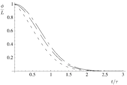
Thus, the characteristic timescale on which the fiber depolymerizes ist (see Appendix 2 for further discussion). It can also be seen that the kinetics is indeed dominated by the large number of depolymerizing ends typically present, peaking at nmax’p ffiffiffix 1 att’t. The evolution of the total

number of fiber ends and the total length of fiber remaining are shown in Figs. 2 and 3, respectively.

Verification of mean-field results by simulation

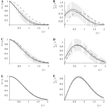
A Monte Carlo simulation routine was constructed to simulate stochastic fiber decomposition. In this routine an initial fiber was permitted to depolymerize deterministically from its ends while the side-depolymeriza-tion, or breaking, events were simulated stochastically with an appropriate breaking probability per unit time. The simulation results, including averages over 1000 simulation runs, are shown in Fig. 4, A–F. These results show that the analytic mean-field solution is remarkably accurate, probably being sufficient for most purposes even forx*10. The stochastic uncertainty represented by the vertical bars in the simulation data are seen to diminish asxincreases. These are not error bars per se but are rather the variation that should be expected between similar realizations of the stochastic depolymerization process. It is seen that the asymptotic-mean field result in thex/Nlimit yields an excellent approximation to both the simulation data and the finitex-mean field results, providedxis large.

The excellent agreement between the mean-field results of the previous section, in which a single characteristic mean fiber length is retained, and those obtained by simulations, which involves the full length distribution, hints that only a single length scale is needed to parameterize the distri-bution. In turn, this suggests that the distribution is monoexponential through-out most of the depolymerization process. This can be confirmed, either by inspection of the length distribution obtained by simulation, or by an ap-proximate analytic approach (R. W. Briehl, unpublished).

COMPARISON WITH EXPERIMENT

Materials and Methods

Differential interference contrast (DIC) microscopy

The Materials and Methods used in this study are as per Agarwal et al. (3) and the reader is referred there for additional technical details. In brief, HbS was purified chromatographically and prepared at 3.75 mM on slides prepared in a glove bag containing from 1% to 100% CO in nitrogen. Fibers and gels were observed at room temperature by video-enhanced differential interference contrast (DIC) microscopy with mercury arc illumination at 546 nm. Deoxygenation and polymerization were induced by photolysis of COHbS by epi-illumination at 436 nm. Once a gel was formed, it was selectively depolymerized by changing epi-illumination intensity (and hence fractional deoxygenation) and the region photolyzed until only an isolated fiber in free solution remained. This procedure of fiber surgery is necessi-tated by the nucleation-dependent nature of gelation: when sufficient inten-sity is used to overcome the high barrier to nucleation, extensive further polymerization occurs very rapidly, with formation of a dense cross-linked gel, precluding creation of individual fibers free of the network. Hence, fibers in free solution cannot be produced in the initial gelation stage; they require selective dissolution of a previously formed gel. After the desired fibers were formed, they were held at constant length within the photolyzed regions to allow solution CO transients to diffuse. The circular photolysis spots were usually 15 but sometimes 25, 10, or 6 mm in diameter. All experiments were at room temperature. Depolymerization in circular spots was initiated by extinguishing the photolytic epi-illumination.

Interpretation

It was already established in an earlier study (3) that fiber end-depolymer-ization rates, as observed under DIC microscopy, vary only slightly with the FIGURE 2 The number of polymer endsnpresent at timetafter the onset

of depolymerization. Shown are the results for finitex, as analyzed in Appen-dix 1,x¼10 (short dashes),x¼100 (long dashes), and the asymptotic behavior in the largexlimit (shortandlong dashes), which gives a good ap-proximation for the overall depolymerization time for all values 1x(L/d)2 as given in Eq. 8.

concentration of CO. The typical end-depolymerization rate is kend

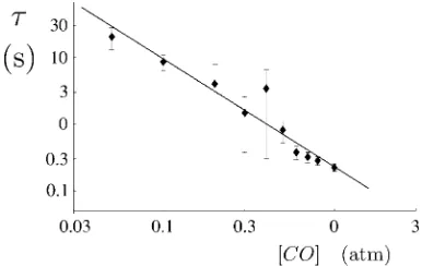
0.5mm/s. The overall timescale on which the fiber disappears is, however, observed to vary substantially. A fully quantitative analysis of this process, including side-depolymerization, is made possible by the combination of theory and experiment reported here. To calculate the variation of the side-depolymerization rate we carried out repeated observations of the depoly-merization of single sickle hemoglobin fibers using DIC video microscopy. This allowed us to estimate the disappearance time of the fiber, after the removal of photolysis, under different CO concentrations; see Fig. 5. As we will now discuss, this provides the first quantitative probe of how the rate of the side-depolymerization process scales with the concentration of CO, acting as a proxy for oxygen. A least-squares fit to the experimental data points of Fig. 5 indicates a slope of1.6, giving the scaling of

kside

;

½

CO

(9)

from Eq. 3. This represents the first quantitative evidence for a substantial cooperative influence of oxygen on the side-depolymerization rate. As discussed in Agarwal et al. (3), in which a limited number of similar experiments were reported, there is some question that CO diffusion may influence the rate for the most rapidly depolymerizing fibers, leading to slower side-depolymerization than the underlying rate at that (bulk) concentration. However, the data shown on Fig. 5, for concentrations [CO]$0.5 atm, were obtained using both a small (21 repeats) and a large (38 repeats) optical photolysis field of 6- and 15-mm diameter, respectively. The fact that there was rather little consistent difference between the two field sizes helps to support the hypothesis that any artifacts associated with the diffusion of CO to the fiber may be rather minor.

Electron microscopy measurements

In this section we reanalyze previously published data. In Fig 8 of Agarwal et al. (3), a fiber is shown in various stages of depolymerization and strongly resembles Fig. 1 of this article. In this case, depolymerization was induced by dilution, rather than CO photolysis (the reader is referred to Agarwal et al. (3) for experimental details). We have no overall timescale for the process of depolymerization, merely a snapshot of the state of the fiber at an unknown time after the onset of depolymerization. Although this means we cannot extract absolute values ofkendandkside, we can estimate their relative values,

as we now demonstrate. The left frame in Fig. 8 of Agarwal et al. (3) shows a fiber withf0.6Lhaving five segments (n¼10) in anL¼1-mm section. From Fig. 3, we havet0.8tand, from Fig. 2,n0:8pffiffiffix. From the definition ofx[ksideL

2

/kendwe have

k

k

160

m

m

_:

(10)

Thus, under these conditions, side-depolymerization plays an important role for any fibers that are longer than;80 nm, corresponding tox*1.

CONCLUSIONS

We have shown how the rate of fiber depolymerization can

depend on the geometric mean of both the end- and

side-depolymerization rates. In particular the timescale for fiber

FIGURE 4 (A–F) The variation of

the total length fraction of remaining fiberf/L(A,C, andE) and the number of ends present, shown the rescaled end density n=pffiffiffix (B, D, and F) as a function of the time after the onset of depolymerization in units of the char-acteristic timescaletdefined in Eq. 3. The curves show the mean-field solu-tion, both for finite values of x as derived in Appendix 1 (solid line) and forx/N; see Eqs. 7 and 8 (dashed line). Also shown is the data from the simulations of the fiber depolymeriza-tion process: the points show the aver-age over 1000 simulations and the vertical bars represent the 1-SD sto-chastic variation for a single realization. Shown arex¼10 (AandB),x¼102

(CandD), andx¼105_{(EandF). It can}

be seen that even forx-values as low as 10 there is good agreement between the mean-field result and the simulation mean and a relatively large stochastic variation about the mean between indi-vidual simulation runs. As the value of

xincreases, we see both that the mean-field estimate asymptotically converges to the mean of the simulations, but that the stochastic variation diminishes as well. This can be understood in terms of the fact that the larger thex, the more breaks a typical fiber experiences, and the better the statistics that emerge from a single simulation run.

Fiber Depolymerization 1011

depolymerization

t

need not depend on the initial length of

the fiber. Our mean-field results for finite values of the

pa-rameter

x

, controlling the relative rate of the side- and

end-depolymerization processes, are fully quantitative, being in

excellent agreement with our corresponding Monte Carlo

simulations. When compared with experiments, our

mean-field results give information about the two kinetic rates

controlling depolymerization. As we have discussed, the

process of depolymerization may play an important role in

the pathology of sickle cell disease. We show that one of the

rates, controlling the formation of new fiber breaks, scales

with roughly the third power of oxygen concentration. Our

theory is actually rather general and should describe the

depolymerization of all linear aggregates that shed

mono-mers from their ends as well as via the formation of short

breaks.

APPENDIX 1: SOLUTIONS TO EQS. 5 AND 6

We can obtain a second-order nonlinear ODE forfby substituting forn from Eq. 5 into Eq. 6,

f

_f

¨

_¼

_2k

side

k

f

₁

_f

_f

_

_:

(11)

We now identify the characteristic timescalet¼1= ffiffiffiffiffiffiffiffiffiffiffiffiffiffiffikendkside p

and use the identitiesf2d

dtfff_

1_{¼ff¨ ff}_2_andfff_ 1_¼d

dtlogfto write the differential equation for logf,

d

dt

log

f

¼

2

=

t

_;

(12)

which has the general solution of

f

¼

A

exp

½ð

t

=

t

Þ

1

B

ð

t

=

t

Þ

;

(13)

and hence, from Eq. 5

n

¼

A

kend

½

2t

=

t

2

₁

B

=

t

exp

½ð

t

=

t

Þ

1

B

ð

t

=

t

Þ

:

(14)

The particular solution of interest to us here is determined by the boundary conditionsf(0)¼Landn(0)¼2 corresponding toA¼LandB¼2=pffiffiffix and hence the solutions (Eqs. 13 and 14) above. However, in the regime

x1 of interest, the solutions are well approximated by Eqs. 7 and 8, as given in the Theory section.

APPENDIX 2: INTERPRETATION OF

THE CHARACTERISTIC FIBER

DEPOLYMERIZATION TIME

t

The fact that the fiber depolymerizes according to Eq. 7 implies that the fiber has substantially depolymerized after a time of the order oft. Indeed, any experimental probe that is sensitive to the length of fiber remaining will register the fiber as having completely disappeared after a few (two, say) timest. Nonetheless, one can ask, What is the terminal fiber depolymer-ization time t* after which the very last fiber segment disappears on average? It is a delicate matter to estimate this timescale from our mean-field approach as our treatment starts to break down in the late stage of depoly-merization, when there are no longer many segments present. Nonetheless, an appropriate estimate can be constructed as follows.

Definet* to be the time at which there is O(1) segment remaining. Thus settingn¼2 in Eq. 8, we have

ð

t

₌

_t

_Þ

_exp

_½ð

_t

₌

_t

_Þ

¼

1

=

p

ffiffiffi

x

:

(15)

This is a transcendental equation for t*/t but is dominated by the exponential term and, neglecting logarithmic corrections, is approximately satisfied when

t

_t

ffiffiffiffiffiffiffiffiffiffi

log

x

2

r

:

(16)

The additional time it takes for this final segment to depolymerize by end-depolymerization alone is of the order of f(t*)/(2kend) t/2, which is

smaller thant* in the regimex 1. Thus we estimate that the fiber completely disappears on the timescalet* which, for all practical values of

x, is not much greater thant. For example, withx¼100 we obtaint*¼ 1.5t from Eq. 16 and find that t* only exceeds 10t for completely unrealistic values ofx.1043.

This work was supported by the National Institutes of Health National Heart, Lung, and Blood Institute program project grant No. HL58512 to R.W.B. (Principal Investigator), F.A.F., and R.J., and grant No. HL22654 to R.J.

REFERENCES

1. Alberts, B., D. Bray, J. Lewis, M. Raff, K. Roberts, and J. Watson. 1994. Molecular Biology of the Cell. Garland, New York.

2. Cates, M. E., and S. J. Candau. 1990. Statics and dynamics of worm-like surfactant micelles.J. Phys. Condens. Matter.2:6869–6892. 3. Agarwal, G., J. C. Wang, S. Kwong, S. M. Cohen, F. A. Ferrone,

R. Josephs, and R. W. Briehl. 2002. Sickle hemoglobin fibers: mech-anisms of depolymerization.J. Mol. Biol.322:395–412.

4. Eaton, W. A., and J. Hofrichter. 1990. Sickle cell hemoglobin poly-merization.Adv. Protein Chem.40:63–279.

5. Ferrone, F. A., J. Hofrichter, and W. A. Eaton. 1985a. Kinetics of sickle hemoglobin polymerization. I. Studies using temperature-jump and laser photolysis techniques.J. Mol. Biol.183:591–610. FIGURE 5 The variation of the lifetime of the fibertwith the

6. Ferrone, F. A., J. Hofrichter, and W. A. Eaton. 1985b. Kinetics of sickle hemoglobin polymerization. II. A double nucleation mecha-nism.J. Mol. Biol.183:611–631.

7. Hogg, J. C., H. O. Coxson, M. L. Brumwell, N. Beyers, C. M. Doesschuk, W. MacNee, and B. R. Wiggs. 1994. Erythrocyte and poly-morphonuclear transit time and concentration in human pulmonary capillaries.J. Appl. Physiol.77:1795–1800.

8. Kolmogorov, A. N. 1937. A statistical theory of metal crystallization. Izv. Akad. Nauk SSSR. Ser. Khem.3:355–359.

9. Avrami, M. 1939. Kinetics of phase change. I. General theory.J. Chem. Phys.7:1103–1112.

10. Shivashakar, G. V., M. Feingold, O. Krichevsky, and A. Libchaber. 1999. RecA polymerization on double-stranded DNA by using single molecule manipulation: the role of ATP hydrolysis.Proc. Natl. Acad. Sci. USA.96:7916–7921.

11. Turner, M. S. 2000. Two time constants for the binding of

proteins to DNA from micromechanical data. Biophys. J. 78:

600–607.

Fiber Depolymerization 1013