An Analytic and Empirical Evaluation of Return on Investment Based Active Learning

An Analytic and Empirical Evaluation of Return-on-Investment-Based

Active Learning

Robbie Haertel, Eric K. Ringger, Paul Felt, Kevin Seppi

Department of Computer Science Brigham Young University

Provo, Utah 84602, USA

[email protected],[email protected], [email protected],[email protected]

Abstract

Return-on-Investment (ROI) is a cost-conscious approach to active learning (AL) that considers both estimates of cost and of benefit in active sample selection. We investigate the theoretical conditions for successful cost-conscious AL using ROI by examining the conditions under which ROI would optimize the area under the cost/benefit curve. We then empirically measure the degree to which optimality is jeopardized in practice when the conditions are violated. The reported experiments involve an English part-of-speech annotation task. Our results show that ROI can indeed successfully reduce total annotation costs and should be consid-ered as a viable option for machine-assisted annotation. On the basis of our experiments, we make recommendations for benefit esti-mators to be employed in ROI. In particular, we find that the more linearly related a benefit estimate is to the true benefit, the better the estimate performs when paired in ROI with an imperfect cost estimate. Lastly, we apply our analysis to help explain the mixed results of previous work on these questions.

1 Introduction

In active learning (AL), a sample selection algorithm sequentially chooses instances, or “samples,” to be labeled/annotated by an oracle. Each annotated stance results in a measurable benefit, such as an in-crease in model accuracy, and incurs a specific cost, such as the time needed to obtain the label. Unfor-tunately some AL research has ignored the fact that

instances have varying costs. Decision-theoretic ap-proaches (e.g., Liang et al., 2009) can incorporate per-instance cost but typically ignore it during ex-perimentation, due in part to the difficulty of sub-tracting cost from benefit when they are measured in different units (Donmez and Carbonell, 2008; Haer-tel et al., 2008). Return-on-investment (ROI) is a cost-conscious technique that avoids this require-ment by selecting the instancex∗_{having maximum}

net benefitper unit cost, i.e.,

x∗=argmax

x

bene fit(x)−cost(x)

cost(x) . (1)

This approach to AL was independently proposed by Donmez and Carbonell (2008), Haertel et al. (2008), and Settles et al. (2008); in addition, Tomanek and Hahn (2010) evaluated the effectiveness of ROI. Un-fortunately, the published results regarding the use-fulness of ROI are mixed. In addition, despite its intuitive appeal as a practical cost-conscious algo-rithm, there has been little theoretical justification for the ROI approach to AL.

The purpose of this paper is to provide an initial theoretical analysis of ROI that, in turn, allows us to identify the conditions needed for the successful application of ROI in a practical environment. We also empirically assess the degree to which violated conditions affect the overall performance of ROI and shed some light on the previously published results. The paper is organized as follows: related work is presented in Section 2. Section 3 examines the con-ditions under which ROI would be optimal. tion 4 discusses the experimental methodology. Sec-tion 5 experimentally assesses the extent to which

the conditions hold in practice – but outside the con-text of AL – while Section 5 explores the overall effect on AL. Finally, Section 6 presents our conclu-sions.

2 Related Work

The essence of active learning is to select the next “best” instance to be annotated. Naturally, the ques-tion arises: which sample selecques-tion funcques-tion is op-timal? Cohn et al. (1996) derive a solution for se-lecting the instance that minimizes model variance. A related class of solutions based on optimal ex-perimental design uses Fisher information to select the optimal instance (Zhang and Oles, 2000). How-ever, these approaches fail to account for problems in which instances are not equally costly to annotate. Decision theory offers an elegant framework for (greedily) selecting the next best instance based on the utility of the instance and considering variable query costs. Some examples include Liang et al. (2009), Anderson and Moore (2005), Margineantu (2005), and Kapoor et al. (2007). In this frame-work, the optimal instance is the one with maximum net utility, that is, utility minus cost. However, this approach requires that utility and cost be measured in the same units. This requirement is particularly problematic when heuristics (such as entropy) are used to approximate expected utility.

Another approach, borrowed from the financial industry, is return-on-investment (ROI) (Donmez and Carbonell, 2008; Haertel et al., 2008; Settles et al., 2008). ROI is related to the decision theo-retic approach (Haertel et al., 2008); however, un-like the decision theoretic approach, ROI does not require conversion between units of utility (benefit) and cost. ROI has explicitly been employed with mixed results on a variety of tasks. Donmez and Car-bonell (2008) show positive results with ROI on face detection, letter recognition, spam detection, and high revenue detection tasks but do not evaluate ROI using variable instance costs. Settles et al. (2008) evaluate ROI on entity-relation tagging, speculative text classification, and information extraction. They limit themselves to an N-best approximation to en-tropy for the sequence labeling tasks, but in this study ROI does not outperform basic AL. Haertel et al. (2008) show positive performance of ROI on

En-glish part-of-speech tagging. Finally, Tomanek and Hahn (2010) find that ROI slightly outperforms two new cost-conscious algorithms when an appropriate benefit function is used.

3 Theoretical Analysis of ROI

The purpose of this section is to provide a bottom-up theoretical explanation of ROI. The analysis also provides a framework within which we can explain why in some previous work ROI has succeeded while in other work it has failed. This section ex-amines Area Under the cost/benefit Curve (AUC) as a suitable objective function and then enumerates a set of conditions that, if true, would lead to ROI maximizing AUC. Within the context of a bottom-up derivation of ROI, the assumptions introduced are somewhat strong, but we dedicate the remainder of the paper to analyzing the degree to which they hold in practice and their effect on practical results.

We begin with a brief set of definitions. AL algo-rithms sequentially select instances from a set of un-labeled instancesU (“the pool”). As an instancex∈ U is annotated with labely, it results in a measur-able benefit and also incurs a specific cost. For the purposes of this section, we follow previous work in assuming a single annotator and in recognizing that the benefit and cost of obtaining a particular anno-tation may depend on previously obtained annota-tions. Thus, we definetotal benefitandcumulative costto be functions (b(·)andc(·), respectively) of a sequence of labeled dataL=h(x1,y1),...,(xn,yn)i.

For simplicity, we assume that the cost to annotate an instance is independent of its place in the se-quence, although it can be shown that this assump-tion has no bearing on the final analysis. Therefore,

c(L1...i) =∑i0c(L_i0).

All previous work of which we are aware eval-uates AL using cost/benefit curves or some deriva-tion thereof. Cost/benefit curves (a generaliza-tion of standard learning curves) parametrically plot

b(L1...i) against c(L1...i) fori∈ {1,...,|L|}. Rather

Osborne (2004) use AUC to evaluate AL algorithms. We now formally define AUC. Assuming linear interpolation between discrete neighboring points, AUC is the sum of the area of the right trapezoids defined by adjacent points on the curve. Letai(L)

be the area of theith_trapezoid:

ai(L) =1₂[c(L1...i)−c(L1...i−1)]

·[b(L1...i−1) +b(L1...i)] (2)

(wherec(/0) =b(/0) =0). Then, the AUC defined by the sequenceLis:

auc(L) =∑_i|₌L|₁ai(L). (3)

Maximizing AUC using AL can be seen as a sequen-tial decision problem in which each decision con-sists of selecting an instance for annotation. The op-timal instance to select given previous annotations

L, will depend on the decision’s effect on the next decision, and the effect of the second decision on the third, and so forth, until all decisions have been made. To account for this recursive dependence, we must consider entire sequences of decisions. Note that if we do not allow instances to be selected more than once fromU we will eventually choose every instance and the number of decisions per sequence isN=|U|.1 _{Additionally, since the actual}

annota-tions that the oracle will provide are unknown, they must be considered in expectation, represented with random variablesYi. Given a sequence of already

an-notated dataL, one approach to maximizing AUC in expectation that accounts for this recursive effect of decisions is (see Haertel et al., 2008 for a decision-theoretic variant):

x∗₁,...,x∗_N=argmax

x1,...,xN

E_{Y1...YN|x1...xN,L}[auc(L⊕ h(x1,y1)...(xN,yN)i)] (4)

where ⊕ represents sequence concatenation. Al-though finding the optimal sequence in this way ac-counts for the effects each decision has on succes-sive decisions, in fact, the sequential decision pro-cess protocol requires only the first instance in this

1_{This limit is rarely reached in practice due to budgetary}

constraints, however, such a constraint does not affect the cur-rent analysis. One simply performs computation as if they were going to annotate all instances, but then only selects the best instance, repeating the process until the budget is exhausted.

sequence, viz.,x∗

1. We then appendx∗1 and the

ora-cle’s annotation for the instancey1 toL. The result

is an updated belief reflected in the expectations (via the newL) used to select the next instance.

We now derive ROI from equation 4 under the fol-lowing conditions:

1. The covariance of cost and benefit is zero. 2. The cost and benefit of each instance are

in-dependent of the order in which instances are annotated.

3. Each random variableyi (i.e., label) is

condi-tionally independent of all otheryj6=i, given xi

andL.

4. Cost and benefit are exact up to a scalar con-stant.

The reader is reminded that we do not necessarily presume these conditions to hold in practice; we briefly discuss their practicality herein and later em-pirically examine the degree to which they hold.

and McCallum, 2001), these approaches are imprac-tical for structured prediction tasks; we will exam-ine the effectiveness of several heuristic benefit esti-mators in our empirical examination. Similarly, al-though cost is sometimes knowablea prioriit often is not. However, Settles et al. (2008) showed that cost can be reliably learned in practice.

While we defer the question of the degree to which these assumptions are violated in practice to our experiments, we proceed with the analysis as if they were true to better understand the theoreti-cal underpinnings of ROI. In the context of maxi-mization, the scalar constants allowed by condition 4 can be ignored. The linearity property of expec-tations allows us to move the expectation in equa-tion 4 inside of the sum in equaequa-tion 3. The first con-dition then allows us to move the expectation further into the area calculation so that equation 2 becomes (omitting expectation indices for brevity):

ai(L) =1₂(E[c(L1...i)]−E[c(L1...i−1)])

·(E[b(L1...i−1)] +E[b(L1...i)]). (5)

Condition 2 implies thatb(L1...i) =∑ii0₌₁b(L_i0);

ap-plying linearity, we obtain:

E[b(L1...i)] = i

∑

i0₌₁Eyi0|x1...i0,y1...i0−1,L[b(Li

0)] (6)

(idem. for cost). Finally, condition 3 implies that:

E[b(L1...i)] = i

∑

i0₌₁Eyi0|xi0,L[b(Li

0)] (7)

(idem. for cost). This result allows us to compute the expected cost and benefit of each instance once per iteration of active learning (as is common outside of decision theoretic frameworks). Because these quantities can be computed independently of one an-other, we can represent each instance xi by a line

segment with fixed width and height—the expected cost and benefit, respectively, according to the cur-rent model—and statically compute the area using these line segments.

It can be proven that, under these conditions, the sequencex∗

1,...,x∗N that maximizes AUC is the

se-quence that is in non-strict slope-non-increasing or-der.2 _{This is precisely the ordering provided by ROI}

2_{A detailed proof sketch is provided by Haertel (2013).}

(see equation 1). Thus, under these conditions, ROI is optimal. (Recall that typically only the first ele-mentx∗

1 is annotated, models are updated, then the

process repeats).

4 Experimental Methodology

In this section, we describe our methodology for em-pirically assessing the degree to which the condi-tions of Section 3 hold in practice and define what we mean by practical contexts. Space constraints limit our experiments to a single task: English part-of-speech (POS) tagging on the POS-tagged Wall Street Journal text in the Penn Treebank version 3 (Marcus et al., 1993).

For this task, we employ Maximum Entropy Markov Models (MEMMs) to model the distribu-tion of tags given words, p(t|w). The model choice is motivated primarily by the speed of retraining. AL typically begins with a small set of randomly selected instances: we use 100 instances annotated “from scratch” (i.e., without AL). However, we do account for the cost incurred by annotating the seed set using the cost simulation described below. Each experiment is run 5 times with a different random seed. For TVE (a committee-based approach; see below), we use a committee size of 5 and train all members in parallel. We additionally score in-stances in parallel, using 4 threads; the remaining processors are used for training the cost model, eval-uating benefit, and garbage collection. For non-committee methods, we found that extra scoring threads do not improve results. All simulations are run on dual hex-core Intel Westmere 2.67 GHz CPUs equipped with 24 GB of RAM.

4.1 Active Learning Simulation

We are interested in empirically testing ROI outside of the clean mathematical environment implied by Section 2. However, the number of experiments we performed necessitated running AL in simulation. Nevertheless, we employ various techniques to keep the simulation as true-to-life as possible.

model assumes that instances are pre-annotated us-ing an automatic annotation model, and the task of the annotator is to correct the errors from the predic-tive model. The length of time required to annotate a sequence w, pre-annotated with hypothesis tags t

and true tagsy, is:

cost(w,y,t) =α+β· |w|+γ·∑_i|y₌|₁1(yi6=ti) (8)

The sum represents the number of tags from the pre-annotation that the annotator changed. We estimate the parameters of the linear model (α=50.534,β=

2.638,γ = 4.440) using the user-study data from Ringger et al. (2008). To add noise to the simulated cost, we generate a random deviate from a shifted Gamma distribution having mean equal to the time predicted by the model, a variance of 5063.35 (the empirical variance of the user-study data), and a shift of 10.0 (near the minimum time). We chose a (shifted) Gamma distribution because the data from the user study appear to be Gamma distributed; as an added benefit, the generated values are guaranteed to always be positive.

In our experiments, we simulate the scenario in which annotators request instances to annotate on demand, e.g., by requesting work on a crowd-sourcing service; we call this annotator-initiated AL. This AL contrasts to the alternative in which the al-gorithm spends time determining the next instance to be annotated and then sends the instance to an annotator to perform the work. We call this lat-ter paradigm learner-initiated AL. The usual implicit assumption in learner-initiated AL is that no cost is incurred between the time the machine sends a re-quest to the annotator and the time the annotator actually starts the work. This assumption is unre-alistic, despite being the approach to AL simula-tion in previous work; real annotasimula-tion projects are annotator-initiated (e.g., crowd-sourcing). The “Par-allel No-Wait” active learning framework introduced by Haertel et al. (2010) follows the more true-to-life annotator-initiated paradigm and provides the guar-antee that annotators never need to wait for an in-stance. We further extend the framework by scoring instances, training the cost model, and training the tagging model in parallel.

Realistic annotation environments also often in-volve multiple annotators (cf. Donmez and Car-bonell, 2008). We take an incremental step towards

allowing multiple annotators by assuming that all annotators are infallible and have the same distribu-tion over the amount of time to annotate any given instance. Under these circumstances, each instance needs to be annotated only once, and annotators are interchangeable. We simulate in real time 20 tire-less oracles who continuously and simultaneously annotate instances for 50 hours each. In contrast to learner-initiated AL, this represents theworst possi-ble case for the no-wait framework since models are maximally out-of-date. Thus, this simulation pro-vides an empirical lower bound on the AUC.

4.2 Cost Estimation

The denominator in ROI is an estimate of the cost to obtain a label for the instance being scored. This estimate is not to be confused with the simulation of annotation times for selected instances, as described in the previous section. The cost estimate (as used in ROI) is computed over many instances to help select an informative instance when the annotator requests one. Once the instance has been selected, we then (noisily) simulate what it would cost for the anno-tator to annotate it, as described above. For algo-rithms that estimate cost as the time to annotate an instance, we learn a linear model of the same form as equation 8. The coefficients are learned using the data obtained during AL (ultimately obtained from the noisy simulation). However, since we do not know which of the automatically pre-annotated tags are incorrect during estimation, we must compute the expected number of incorrect tags in place of the sum in equation 8.

The results of our experiments are potentially better than in practice since our cost estimate has exactly the same form as the simulated true cost. However, the results are still useful because (1) the gamma-distributed noise in the true cost has high variance and (2) the estimate is computed in expec-tation (using the learned model).

4.3 Benefit Estimation

ROI’s numerator is an estimate of the benefit of ob-taining a label for a given instance. As previously mentioned, optimal benefit estimators are imprac-tical for structured learning problems; uncertainty-based heuristics are typically employed instead. Let

sen-tencew. Drawing mostly from previous studies, we consider the following:

Constant (CONST) assumes all instances have

equal benefit.

Approximate Token Entropy (ATE) (Settles

and Craven, 2008) approximates the true sequence entropy as the sum of the entropy of the individual marginal distributions p(ti|w). The marginal

distri-butions can in turn be approximated as p(ti|w)≈

p(ti|t_i∗₋₁,w) where ti∗−i is the (i−1)th tag in the

Viterbi best sequencet∗_{; a beam search can}

signifi-cantly reduce computation.

Monte Carlo Entropy (MCE) uses a Monte

Carlo approximation to compute the entropy, i.e.,

E[−logp(t|w)], using samples taken from t|w(the

trained MEMM).

N-best Sequence Entropy (NSE) (Settles and

Craven, 2008) approximates sequence entropy by computing the entropy of the top-n sequences, where the probabilities are re-normalized to sum to unity.

Least Confidence (LC)(Culotta and McCallum,

2005), in contrast to entropy, is not concerned with the distribution over the entire support, but rather fo-cuses on the best option and its complement (the rest of the support). It is the probability of being wrong, i.e., 1−maxtp(t|w).

Negative Max Log Probability (NMLP)

(Haer-tel et al., 2010) is defined as −maxtlogp(t|w); it ranks instances the same as LC but with different scores under the assumption that the relationship be-tween probabilities and change in accuracy is loga-rithmic rather than linear.

Token Vote Entropy (TVE) (Engelson and

Da-gan, 1996) uses a committee of classifiers trained from bootstrapped samples of the annotated data. For each word, each committee member votes for the tag it predicts for its word; the entropy of the distribution over votes is summed over each word in the sentence.

5 From Theory to Practice: To What Degree Are the Conditions Met?

In this section, we empirically test some of the ditions from the preceding analysis in practical con-texts. For the purposes of this work, we are mostly interested in examining conditions 1 and 4. While

condition 3 (conditional independence) is assumed in most previous work, we leave quantification of the effects of violating this condition and the related condition 2 to future work.

For these experiments, it is necessary to estimate true benefit and cost. Due to the complexity of so doing, we compute the various metrics along a pas-sivelearning curve (i.e., without AL). We compute the true cost of each instance as described in Sec-tion 4.1. In order to estimate the true benefit of a par-ticular instance at a parpar-ticular point on the learning curve, we assume that the true benefit of an instance is the change in held-out accuracy that would result from incorporating the instance with its annotation into the training data; we ignore the effects of future choices. We compute the change in accuracy (ben-efit) by adding the instance and its true label to the training data, retraining the model, and then com-puting the model’s new accuracy on the held-out set. The process is repeated to compute the true benefit of at least 1,000 instances and the statistics noted be-low are averaged over 5 random initial training sets. We use one standard error as a simple measure of statistical significance.

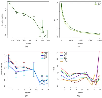
Is the covariance of cost and benefit zero? Us-ing the aforementioned methodology, we compute Pearson’s correlation coefficient (a normalized form of covariance) between benefit and cost. As seen in figure 1a, true benefit and cost have virtually no correlation when model quality is high, and is only weakly correlated in the early stages. Thus, condi-tion 1 roughly holds.

To what extent is the cost estimate a scalar mul-tiple of true cost? Using the technique mentioned above, we produce pairs of true cost and estimated cost at various locations along the learning curve and computeR2 _{values of a linear model estimated}

with they-intercept fixed at zero. Pearson’s corre-lation coefficient is inappropriate since it would al-low for the cost estimate to be shifted in addition to being scaled. AnR2 _{of 1.0 would indicate that}

(a) (b)

(c) (d)

Figure 1: At various points on the learning curve: (a) correlation between true cost and true benefit (b)R2

values representing the degree to which the cost estimate is a scalar multiple of the true cost, for varying amounts of variance in the noise model at two points on the learning curve (83% and 96%). (c)R2 _values

representing the degree to which various benefit estimators are scalar multiples of true benefit (d) POMAS of the top-20 instances. Error bars represent one standard error.

as variance increases underscores the importance of accounting for as much variance as possible in the cost model. We found the R2 _{values to be around}

0.745 and 0.785 when the variance was equal to that of the aforementioned user study (and the one used through the remainder of the experiments). We note that these numbers may be overly optimistic given the similarity between the model used to simulate annotation times and that used to estimate cost. As a point of reference, Settles et al. (2008) and Arora

and Nyberg (2011) reportR2 _{values for cost}

mod-els fordifferenttasks on the order of 0.3–0.4. Even these values indicate some scalar relationship be-tween true and estimated cost as per condition 4.

To what extent are various benefits estimators scalar multiples of true benefit? We repeat the experiment described for cost, but reporting theR2

cost estimate, they are still reasonable. Most of the separation of algorithms (where it exists statis-tically) occurs during the beginning stages of learn-ing. NMLP has a slight (though not statistically sig-nificant) advantage over ATE and MCE while all three are more linearly related to true benefit than NSE and LC. Once the model achieves 91% accu-racy, there is no separation. The results suggest that condition 4 holds weakly for benefit estimators.

Are instances with the highest slopes being se-lected?The success of ROI depends on its ability to select the instance with the highest slope. Using the aforementioned setup, we compute the largest slope of the candidate instances on the basis of estimated benefit and cost and divide it by the largest slope ac-cording to the true values; we call this value the Per-centage of Maximum Attainable Slope (POMAS). Since multiple instances can be selected using the same model in the no-wait framework, we repeat this procedure for the second highest slopes, etc., for the top-20 slopes and average them. The results are in Figure 1d. The separation between algorithms at the beginning mirror those of Figure 1c. We note that there is ample room for improvement even amongst the best algorithms we tried.

6 Active Learning Results and Discussion

The previous experiments were conducted outside of the context of AL in order to gain insight into how well the conditions of section 2 are met in practice. However, the most direct evaluation is the compar-ison of the actual quantity of interest, AUC, in the type of practical AL defined above. We compare normalized AUC (expected benefit) for several ben-efit estimators and two cost estimates and discuss the results in light of the previous section and the theory from Section 2.

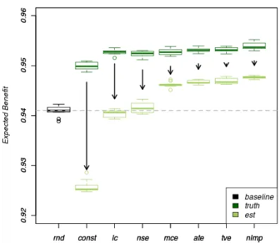
Although not predicted by the theory per se, we would expect AUC to decrease with degrada-tions in the cost and/or benefit estimates. First, we compare the AUC when using the true cost in the ROI calculations (thus satisfying one half of condition 4) and compare the results to using esti-mated cost learned during AL. The results are dis-played in Figure 2. Interestingly, when cost is ex-actly known (perfectly predictable), all estimators– even CONST–readily outperform the random

base-Figure 2: Expected benefit (normalized AUC) for various benefit estimators with true and estimated costs. The median baseline performance (rnd) is depicted as a dashed line and is the same for both experiments. Estimated cost affects the benefit esti-mates to different degrees.

line. Furthermore, the difference between most of the estimators (except perhaps CONST) is not sta-tistically significant, which suggests that a good cost estimate may be capable of overcoming deficiencies in even very poor benefit estimators like CONST. Not surprisingly, all algorithms perform worse when using the learned estimate of cost during AL (in-dicated by the downward arrows), even though the MSE of the learned cost models was high–on the or-der of the variance in the simulated times.

distributions and renormalization makes scores very similar to each other—even for instances of differing lengths. Similarly, although LC and NMLP would rank instances the same (before dividing by cost; di-viding by cost alters the rankings), thelogin NLMP produces greater spread in the score. Since the cost estimates are better dispersed, they tend to dominate ROI for these “low-spread” benefit estimators. To illustrate, consider the extreme case of CONST by substituting an arbitrary constant for benefit in equa-tion 1: instances are selected lowest-expected-cost first. On our particular task, this scenario is particu-larly undesirable as the shortest sentences are nearly always the cheapest but disproportionately informa-tion poor (a contributing factor to the non-zero cor-relation). In more general terms, as the spread in the benefit estimates approaches zero (as in CONST), the cost estimates increasingly become the discrim-inating factor. While this behavior is correct for perfect benefit and cost estimates, it is problematic when condition 4 is violated.

The results also highlight the fact that expen-sive scoring algorithms are naturally penalized in annotator-initiated AL. The relatively expensive sampling in MCE leads to slightly lower perfor-mance than cheaper entropy estimates (ATE); the relatively cheap NMLP outperforms TVE, which in-curs the expense of multiple models.

The mixed results of previous work are explain-able based on our analysis. While condition 4 re-quiresthat cost and benefit estimators be scalar mul-tiples of the true values, our empirical results sug-gest that better estimates yield higher AUC. We have explained why NSE has poor mathematical prop-erties for structured learning tasks and is therefore expected to produce relatively low AUC, hence the negative results on the structured prediction tasks of Settles et al. (2008). In contrast, the authors report positive results on a standard classification problem using exact entropy calculations, coincid-ing with our results in which the good (i.e., non-NSE) entropy estimators are good estimators. We have also explained the poor properties of LC for structured prediction; the results of Tomanek and Hahn (2010) present further empirical evidence. In-terestingly, they find that exponentiating LC leads to positive results. Mathematically,exp(β(1−p)) be-haves similarly to−log(p)(NLMP) in that they both

separate scores that are close together—the former much more so than the latter, especially for proba-bilities of the very low magnitudes seen in structured prediction problems. This separation gives the ben-efit estimate more influence relative to cost as com-pared to LC. In sum, the negative results of previous work are due to poor benefit estimators, in particular LC and NSE; in contrast, positive results are due to better benefit estimators.

7 Conclusions and Future Work

ROI-based AL successfully reduces annotation costs in practice by maximizing the area under the cost/benefit curve. We have provided an initial the-oretical justification for ROI-based AL in a bottom-up fashion. We have shown empirically that, for our task, true benefit and cost have little-to-no correla-tion when model quality is high; cost estimates have a scalar relationship to true cost; similarly for benefit estimates, though to a lesser degree; and the estima-tors that demonstrated the most scalar relationships to the truth resulted in higher AUC.

Although we focused our empirical analysis on a single task, other studies have applied ROI to several tasks and problem types, and their results are consis-tent with our analysis. As a result of this work, we recommend that practitioners carefully select their benefit and cost estimators, ensuring that they are “good” estimators for their task as described above. Particular attention should be paid to the cost esti-mator: even trivial benefit estimators out-performed random with a perfect cost estimator. Also note that estimators (e.g. NSE and LC) that produce scores with relatively little “spread” should be avoided. Fu-ture work could consider using a small set of anno-tated data to estimate how scalar the relationship of the estimators are to true benefit and cost before an-notation begins.

References

Brigham Anderson and Andrew Moore. 2005. Active learning for hidden Markov models: Objective func-tions and algorithms. InProceedings of the 22nd In-ternational Conference on Machine Learning, pages 9–16.

Shilpa Arora and Eric Nyberg. 2011. Assessing benefit from feature feedback in active learning for text clas-sification. InProceedings of the Fifteenth Conference on Computational Natural Language Learning, pages 106–114. Association for Computational Linguistics. Jason Baldridge and Miles Osborne. 2004. Active

learn-ing and the total cost of annotation. Proceedings of the Conference on Empirical Methods in Natural Lan-guage Processing.

David A. Cohn, Zoubin Ghahramani, and Michael I. Jor-dan. 1996. Active learning with statistical models.

Journal of Artificial Intelligence Research, 4:129–145. Aron Culotta and Andrew McCallum. 2005. Reducing labeling effort for structured prediction tasks. In Pro-ceedings of the National Conference on Artificial In-telligence, volume 20, page 746.

Pinar Donmez and Jaime G. Carbonell. 2008. Proac-tive learning: Cost-sensiProac-tive acProac-tive learning with mul-tiple imperfect oracles. InProceeding of the 17th ACM Conference on Information and Knowledge Manage-ment, pages 619–628. ACM.

Sean P. Engelson and Ido Dagan. 1996. Minimizing manual annotation cost in supervised training from corpora. In Proceedings of the 34th Annual Meeting on Association for Computational Linguistics, pages 319–326.

Robbie A. Haertel, Kevin D. Seppi, Eric K. Ringger, and James L. Carroll. 2008. Return on investment for ac-tive learning. InProceedings of the Neural Informa-tion Processing Systems Workshop on Cost Sensitive Learning.

Robbie Haertel, Paul Felt, Eric Ringger, and Kevin Seppi. 2010. Parallel active learning: Eliminating wait time with minimal staleness. In Proceedings of the HLT-NAACL 2010 Workshop on Active Learning for Nat-ural Language Processing, pages 33–41. Association for Computational Linguistics.

Robbie A. Haertel. 2013. Practical Cost-Conscious Active Learning for Data Annotation in Annotator-Initiated Environments. dissertation, Brigham Young University.

Ashish Kapoor, Eric Horvitz, and Sumit Basu. 2007. Se-lective supervision: Guiding supervised learning with decision-theoretic active learning. InProceedings of the International Joint Conferences on Artificial Intel-ligence.

Percy Liang, Michael I. Jordan, and Dan Klein. 2009. Learning from measurements in exponential families. InProceedings of the 26th Annual International Con-ference on Machine Learning, pages 641–648. ACM. Mitchell P. Marcus, Mary Ann Marcinkiewicz, and

Beat-rice Santorini. 1993. Building a large annotated cor-pus of English: The Penn Treebank. Computational Linguistics, 19(2):313–330.

Dragos D. Margineantu. 2005. Active cost-sensitive learning. In Proceedings of the International Joint Conferences on Artificial Intelligence, volume 19, page 1622.

Eric Ringger, Marc Carmen, Robbie Haertel, Kevin Seppi, Deryle Londsale, Peter McClanahan, James Carroll, and Noel Ellison. 2008. Assessing the costs of machine-assisted corpus annotation through a user study. InProceedings of the International Conference on Language Resources and Evaluation.

Nicholas Roy and Andrew McCallum. 2001. Toward optimal active learning through sampling estimation of error reduction. In Proceedings of the Eighteenth International Conference on Machine Learning, pages 441–448.

Burr Settles and Mark Craven. 2008. An analysis of ac-tive learning strategies for sequence labeling tasks. In

Proceedings of the Conference on Empirical Methods in Natural Language Processing, pages 1070–1079. Association for Computational Linguistics.

Burr Settles, Mark Craven, and Lewis Friedland. 2008. Active learning with real annotation costs. In Proceed-ings of the Neural Information Processing Systems Workshop on Cost-Sensitive Learning, pages 1069– 1078.

Katrin Tomanek and Udo Hahn. 2010. A comparison of models for cost-sensitive active learning. In Proceed-ings of the 23rd International Conference on Compu-tational Linguistics: Posters, pages 1247–1255. Asso-ciation for Computational Linguistics.