Inferring the location of authors from words in their texts

Inferring the location of authors from words in their texts

Max Berggren & Jussi Karlgren Gavagai & KTH

Stockholm

{max, jussi}@gavagai.se

Robert ¨Ostling & Mikael Parkvall Dept of Linguistics

Stockholm University

{robert, parkvall}@ling.su.se

Abstract

For the purposes of computational dialec-tology or other geographically bound text analysis tasks, texts must be annotated with their or their authors’ location. Many texts are locatable but most have no ex-plicit annotation of place. This paper describes a series of experiments to de-termine how positionally annotated mi-croblog posts can be used to learn loca-tion indicating words which then can be used to locate blog texts and their authors. A Gaussian distribution is used to model the locational qualities of words. We in-troduce the notion of placeness to describe how locational words are.

We find that modelling word distributions to account forseveral locations and thus several Gaussian distributions per word, defining a filter which picks out words with high placeness based on their local distributional context, and aggregating lo-cational information in acentroidfor each text gives the most useful results. The re-sults are applied to data in the Swedish language.

1 Text and Geographical Position

Authors write texts in a location, about some-thing in a location (or about the location itself), reside and conduct their business in various lo-cations, and have a background in some location. Some texts are personal, anchored in the here and now, where others are general and not necessar-ily bound to any context. Texts written by au-thors reflect the above facts explicitly or implicitly, through explicit author intention or incidentally. When a text is locational, it may be so because the author mentions some location or because the author is contextually bound to some location. In

both cases, the text may or may not have explicit mentions of the context of the author or mention other locations in the text.

For some applications, inferring the location of a text or its author automatically is of interest. In this paper we show how establishing the location of a text can be done using the locational qualities of its terminology. Here, we investigate the utility of doing so for two distinct use cases.

Firstly, for detecting regional language usage for the purposes of real-time dialectology. The is-sue here is to find differences in term usage across locations and to investigate whether terminologi-cal variation differs across regions. In this case, the ultimate objective is to collect sizeable text collections from various regions of a linguistic area to establish if a certain term or turn of phrase is used more or less frequently in some specific re-gion. The task is then to establish where the author of a text originally is from. This has hitherto been investigated by manual inspection of text collec-tions. (Parkvall 2012, e.g.)

Secondly, for monitoring public opinion of e.g. brands, political issues, or other topic of inter-est. In this case the ultimate objective is to find whether there is a regional variation for the occur-rence of opinionated mentions for the topic or top-ical target under consideration. The task is then to establish the location where a given text is written, or, alternatively, what location the text refers to.

of interest in a location, modelling the geographic distribution of topics, or using social network anal-ysis to find additional information about the au-thor.

This set of experiments focuses on the text itself and on using distributional semantics to refine the set of terms used for locating a text.

2 Location and words as evidence of locations

Most words contribute little or not at all to posi-tioning text. Some words are dead giveaways: an author may mention a specific location in the text. Frequently, but not always, this is reasonable ev-idence of position. Some words are less patently locational, but contribute incidentally, such as the name of some establishment or some characteris-tic feature of a location.

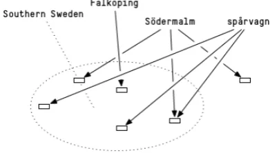
Some locational terms are polysemous; some inspecific; some are vague. As indicated in Fig-ure 1, the termFalk¨opingunambiguously indicates a town in Southern Sweden, which in turn is a vague term without a clear and well defined border to other bits of Sweden. The term S¨odermalmis polysemous and refers to a section of town in sev-eral Swedish towns; the term sp˚arvagn (“tram”) is indicative of one of several Swedish towns with tram lines. We call both of these latter types of termpolylocationaland allow them to contribute to numerous places simultaneously.

Other words contribute variously to location of a text. Some words are less patently locational than named places, but contribute incidentally, such as the name of some establishment, some characteristic feature of a location, some event which takes place in some location, or some other topic the discussion of which is more typical in one location than in another. We will estimate the placenessof words in these experiments.

Figure 1: Some terms are polylocational

3 Mapping from a continuous to a discrete representation

We, as has been done in previous experiments, collect the geographic distribution of word us-age through collecting microblog posts, some of which have longitude and latitude, from Twit-ter. Posts with location information are distributed over a map in what amounts to a continuous repre-sentation. The words from posts can be collected and associated with the positions they have been observed in.

First experiments which use similar training data to ours have typically assigned the posts and thus the words they occur in directly to some rep-resentation of locations - a word which occurs in tweets at [N59.35,E18.11] and[N59.31,E18.05]

will have both observations recorded to be in the same city (Cheng et al. 2010; Mahmud et al. 2012). An alternative and later approach by e.g. Priedhorsky et al. (2014) is to aggregate all obser-vations of a word over a map and assign a named location to the distribution, rather than to each ob-servation, deferring the labeling to a point in the analysis where more understanding of the term distribution is known.

Another approach is to modeltopicsas inferred from vocabulary usage in text across their geo-graphical distribution, and then, for each text, to assess the topic and thus its attendant location visavi the topic model most likely to have gener-ated the text in question (Eisenstein et al. 2010; Yin et al. 2011; Kinsella et al. 2011; Hong et al. 2012). We have found that topic models as imple-mented are computationally demanding, and the reported results show that they do not add accu-racy to prediction. Since they build on a hidden level of ”topic” variables they have little explana-tory value to aid the understanding of localised language use.

4 Test Data

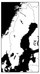
These experiments have focused on Swedish-language material and on Swedish locations. Most Swedish-speakers live in Sweden; Swedish is mainly written and spoken in Sweden and in Fin-land. Sweden is a roughly rectangular country of about 450 000 km2 as shown in Figure 2. Swe-den has since 1634 been organised into 22 coun-ties orl¨anof between 3 000km2and 100 000km2. The median size of a county is 10 545km2which would, assuming quadratic counties, give a side of 100kmfor a typical county.

We measure accuracy of textual location using the Haversine distance, the great-circle distance between two points on a sphere. We report aver-ages, both mean and median, as well as percentage of texts we have located within 100kmfrom their known position.

Our test data set is composed of social me-dia texts from two sources. One set is 18 GB of blog text from major Swedish blog and forum sites, with self-reported location by author - vari-ously, home town, municipality, village, or county. The texts are mainly personal texts with authors of all ages but with a preponderance of pre-teens to young adults. The data are from 2001 and onward, with more data from the latest years. The data are concatenated into one document per blog, to-talling to 154 062 documents from unique sources. Somewhat more than a third, 35%, have more than 10k characters.

The other set is 37 GB of blog text without any explicit indication of location. A target task for these experiments is to enrich these 37 GB of non-located data with predicted location, in order to address data sparsity for unusual dialectal linguis-tic items.

Figure 2: Map of Sweden

5 Baseline: theGAZETTEERmodel

For a list of known places we used a list1of 1 956 Swedish cities and 2 920 towns and villages as de-fined by Statistics Sweden2in 2010.

As the most obvious baseline, we identify all kens found in this list, or gazetteer. Each such to-ken is converted to a position through the Geoen-coding API offered by Google3. The position with largest observed frequency of occurrence in the text is assumed to be the position of the text. Other approaches have taken this as a useful approach for identifying features such as Places of Interest mentioned in texts (Li et al. 2014). We call this approach the GAZETTEERapproach.

6 Training Data

As a basis for learning how words were used we used geotagged microblog data from Twitter. About 2% of Swedish Twitter posts have latitude and longitude explicitly given,4 typically those that have been posted from a mobile phone. We gathered data from Twitter’s streaming API dur-ing the months of May to August of 2014, savdur-ing posts with latitude and longitude and with Sweden explicitly given as point of origin. This gave us 4 429 516 posts of about 630 MB.

7 Polylocational Gaussian Mixture Models

Given a set of geographically located texts, we record for each linguistic item – meaning word, in these experiments – the locations from the meta-data of every text it occurs in. This gives each word a mapped geographic distribution of latitude-longitude pairs. We model these observed distri-butions using Gaussian 2-D functions, as defined by Priedhorsky et al. (2014). A 2-D Gaussian function will assume a peak at some position and allow for a graceful inclusion of hits at nearby po-sitions into the model in a bell-like distribution.

1_{http://en.wikipedia.org/wiki/List of urban areas in Sweden} One named location (“N¨ar”) was removed from the list since it is homographic to the adverbials corrresponding to the Englishnearandwhen, causing a disproportionate amount of noise.

2_{A locality consists of a group of buildings normally not} more than 200 metres apart from each other, and must fulfil a minimum criterion of having at least 200 inhabitants. De-limitation of localities is made by Statistics Sweden every five years.[http://www.scb.se]

3_{https://developers.google.com/.../geocoding/}

Many distributions could be envisioned here, but Gaussians have attractive implementational qual-ities and have a straightforward interpretation in terms of mapping to physical space.

In contrast to the original definition and and other similar following approaches, we want to be able to handle polylocational words. After testing various models on a subset of our data we find that fitting more than one Gaussian function—in ef-fect, assuming that locationally interesting words refer to several locations–yields better results than fitting all locational data into one distribution. Af-ter some initial parameAf-ter exploration as shown in Figure 3, we settle on three Gaussian functions as a reasonable model: words with more than three distributional peaks are likely to be of less utility for locating texts. We consequently fit each word with three Gaussian functions to allow a word to contribute to many locations for the texts it is ob-served in.

1 2 3 4 5 6 7 8

Number of gaussians

0 100 200 300 400 500 600

Error (km)

Mean 25th percentile 75th percentile 50th percentile

Figure 3: Effect of polylocational representations

8 The notion of placeness

In keeping with previous research on geoloca-tional terms such as Han et al. (2014), we rank candidate words for their locational specificity. From the Gaussian Mixture Model representation, we take the log probability ρ in the mean of the Gaussian and transform it into a placenessscore by p=e100−ρ. This is done for every word, for all

three Gaussians. The score is then used to rank words for locational utility.

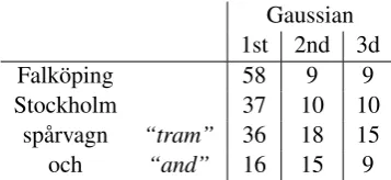
Gaussian 1st 2nd 3d

Falk¨oping 58 9 9

Stockholm 37 10 10

sp˚arvagn “tram” 36 18 15

och “and” 16 15 9

Table 1: Example words and their log placeness

Table 1 shows the placeness of the three Gaus-sians for some sample words. The two sample named locations have high placeness for their first Gaussians, indicating that they have locational utility. “Stockholm”, the capital city, which is frequently mentioned in conversations elsewhere has less placeness than has “Falk¨oping”, a smaller city. The word “tram” has lower placeness than the two cities, and the word “and” with a log place-ness score of 16 can not be considered locational at all. Inspecting the resulting list as given in Ta-ble 2 which shows some examples from the top of the list, we find that words with high placeness frequently are non-gazetteer locations (“Slottssko-gen”), user names, hash tags – frequently refer-ring to events (“#lundakarneval”), and other lo-cal terms, most typilo-cally street names (“Holgers-gatan”), spelling variants (“St˚ackh˚alm”), or public establishments.

The performance of the predictive models intro-duced below can be improved by excluding words with low placeness from the centroid. This exclu-sion threshold is referred to asT below.

known places hash tags other hogstorp #lundakarneval holgersgatan nyhammar #bishopsarms margreteg¨ardeparken

sjuntorp #gothenburg uddevallahus tyringe #westpride14 kampenhof slottsskogen #swedenlove1dday st˚ackh˚alm

storvik #sverigemotet gullmarsplan charlottenberg #sthlmtech tv¨arbanan

Table 2: Example words with high placeness

9 Experimental settings: theTOTALand FILTEREDmodels

We run one experimental setting with all words of a set, only filtered for placeness. We call this ap-proach the TOTALapproach.

nästkusin - hits: 318

None Low Medium High Very high

småkusin - hits: 156

None Low Medium High Very high

tremänning - hits: 589

None Low Medium High Very high

syssling - hits: 1870

None Low Medium High Very high

(a) Using labeled data set

nästkusin - hits: 959

None Low Medium High Very high

småkusin - hits: 678

None Low Medium High Very high

tremänning - hits: 1717

None Low Medium High Very high

syssling - hits: 7204

None Low Medium High Very high

(b) Using enriched data set increases the data

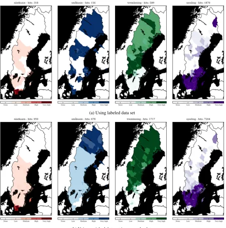
Figure 5: Regional terminology for “second cousin”

linguistic items, we bootstrap from the gazetteer and collect the most distinctive distributional texts of gazetteer terms. For this, we used con-text windows of six words before (6+0), around (3+3), and after (0+6) each target word. These context windows were tabulated and the most fre-quently occurring constructions5 are then ranked based on their ability to return words with high placeness. For each construction, the percentage of words returned with logT >20 is used as a ranking criterion. Using this ranking, the top 150 constructions are retained as a paradigmatic filter

5_{In these experiments, the 900 most frequent} construc-tions are used.

to generate usefully locational words. Construc-tions such aslives in <location>will be at the top of the list as shown in Figure 8.

Words found in the <location> slot of the constructions are frequency filtered with respect to N, the length of the text under analysis, with thresholds set by experimentation to 0.00008×

100 200 300 400 500 600 700 800 900 1000 1100 1200 1300 1400

Error (km)

0.000

0.001

0.002

0.003

0.004

0.005

0.006

Fraction of tests

log(T)=60 log(T)=50 log(T)=40 log(T)=20 log(T)=10 T=0

Figure 6: Comparing placeness thresholds for the FILTEREDCENTROIDmodel.

Placeness Error (km) Percentile (km) e<100km logT e˜ e¯ 25 % 50 % 75 % Precision Recall

FILTEREDCENTROID — 204 365 45 204 464 0.38 0.38

FILTEREDCENTROID 10 204 365 45 204 464 0.38 0.38

FILTEREDCENTROID 20 200 365 44 200 460 0.38 0.38

FILTEREDCENTROID 40 145 333 32 145 396 0.44 0.32

FILTEREDCENTROID 50 90 286 22 90 321 0.52 0.23

FILTEREDCENTROID 60 70 271 13 70 330 0.53 0.04

Table 3: Comparing placeness thresholds for the FILTEREDCENTROIDmodel.

100 200 300 400 500 600 700 800 900 1000 1100 1200 1300 1400

Error (km)

0.0000

0.0005

0.0010

0.0015

0.0020

0.0025

0.0030

0.0035

0.0040

Fraction of tests

Filtered centroid

Filtered vote

Total

Gazetteer

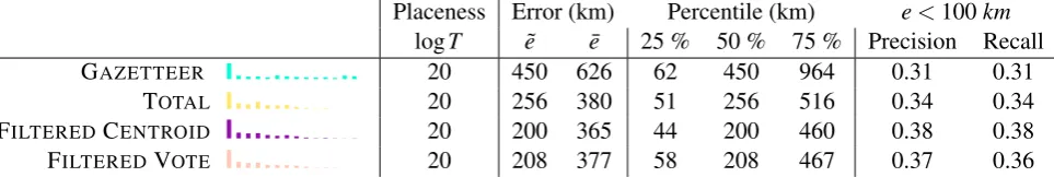
Figure 7: Comparing models with placeness threshold at logT =20.

Placeness Error (km) Percentile (km) e<100km logT e˜ e¯ 25 % 50 % 75 % Precision Recall

GAZETTEER 20 450 626 62 450 964 0.31 0.31

TOTAL 20 256 380 51 256 516 0.34 0.34

FILTEREDCENTROID 20 200 365 44 200 460 0.38 0.38

FILTEREDVOTE 20 208 377 58 208 467 0.37 0.36

(a) All words of a text contribute to the pre-dicted location .

(b) Only words filtered through the distribu-tional model contribute votes to yield a pre-diction very close to the correct position .

Figure 4: Comparison of grid and grammar.

10 Aggregating the locational information for filtered texts

The filtered texts are now processed in two differ-ent ways. Every unique word token in the Twitter dataset has a Gaussian mixture model ibased on its observed occurrences, as shown in Section 8. This is represented by the three mean coordinates µiand their correspondingplacenesses pi.

µi=



 µ1

µ2

µ3



 i

pi=





p1 p2 p3



 i

We compute a centroid for these coordinates, as an average best guess for geographic signal for a text. We do this with an arithmetic weighted mean. Givennwords:

<location> mellan varit i <location> bor i <location> var i <location> vi till <location> in till <location> ska till <location> <location> centrum av till <location> det av till <location> hemma i <location> till <location> upp till <location>

(a) In Swedish

<location> between been in <location> live(s) in <location> was in <location> we to <location> in to <location> going to <location> <location> centre off to <location> go to <location> home in <location> to <location> up to <location>

(b) Translated to English

Figure 8: Examples of locational constructions

M=

n

∑

i=1

µn·pn

n

∑

i=1 3

∑

j=1 pn_j

Whereµn·pn is the dot product6_{. We call this}

model FILTERED CENTROID

Alternatively, we do not average the coornates, but select by weighted majority vote. We di-vide Sweden into a grid of roughly 50x50km cells. The placeness score of every locational word in a text is added to its cell. The centerpoint of the cell with highest score is assigned to the text as a loca-tion. We call this model FILTEREDVOTE.

Figure 4 shows how filtering improves results, here illustrated by the FILTERED VOTE model. The top map shows how every word of a text con-tributes votes, weighted by their placeness, to give a prediction ( ). The bottom map shows how when only words filtered through the distributional model are used, the voting yields a correct result in comparison with the gold standard ( ) given by the metadata.

11 Results

As shown in Table 4 and Figure 7, the Gaussian models FILTERED CENTROID and FILTERED VOTE outperform the GAZETTEER model handily. Filtering words distributionally, in addition to reducing processing, improves results further. The FILTERED CENTROID model is slightly better than the FILTERED VOTE

model , providing support for late discretization of locational information. A closer look at the effect, shown in Table 3 and in Figure 6, of feature selection with the placeness threshold shows the precision-recall tradeoff

6

contingent on reducing the number of accepted locational words.

These results are well comparable with the re-sults reported by others: while direct compari-son with other linguistic and geographic areas is difficult, Cheng et al. (2010) set a 100-mile (≈

160 km) success criterion for a similar task of geo-locating microblog authors (not single posts). They find that about 10% of microblog users can be localised within their 100-mile radius. Eisen-stein et al. (2010) found they could on average achieve a 900 km accuracy for texts or a 24% ac-curacy on a US state level.

12 Regional variation

Returning to our use case we now use the FIL

-TERED CENTROID model to posi-tion and thus enrich a further 38% of our unla-beled blog collection with a location tag (setting the placeness threshold logT =20). This gives a noticeably better resolution for studying regional word usage as shown in Figure 5: the term for “second cousin” varies across dialects, and given the enriched data set we are able to gain better fre-quencies and a more distinct image of usage.

13 Conclusions

Our results show that inferring text or author lo-cation can be done with few knowledge sources. Given a list of known places and microblog posts with locational information we were able to pin-point the location of more than a third of blog texts within 100 kms of their known point of origin. The notable results are three.

Firstly, that locational models trained on one genre can be used for inferring location of texts from another very different genre.

Secondly, that modelling words polylocation-ally (in the present case, using three locations) al-lowed us to use more diverse words than otherwise would have been possible.

Thirdly, that filtering the words by distributional qualities improved results. This point is useful to note even if other approaches than learning loca-tion from posiloca-tioned texts is used: any gazetteer could be used to bootstrap locational constructions and to harvest other candidate terms from texts to enrich it.

Acknowlegdments

This work was in part supported by the grant SI-NUS (Spridning av innovationer i nutida sven-ska) from Vetenskapsr˚adet, the Swedish Research Council.

References

Lars Backstrom, Jon Kleinberg, Ravi Kumar, and Jasmine Novak. Spatial variation in search engine queries. In17th international conference on World Wide Web. ACM, 2008. Zhiyyan Cheng, James Caverlee, and Kyumin Lee. You are where you tweet: a content-based approach to geo-locating Twitter users. In19th ACM international Confer-ence on Information and Knowledge Management. ACM, 2010.

Jacob Eisenstein, Brendan O’Connor, Noah A Smith, and Eric P Xing. A latent variable model for geographic lexical variation. InConference on Empirical Methods in Natural Language Processing. ACL, 2010.

Bo Han, Paul Cook, and Timothy Baldwin. Text-based Twit-ter user geolocation prediction.Journal of Artificial Intel-ligence Research (JAIR), 49:451–500, 2014.

Liangjie Hong, Amr Ahmed, Siva Gurumurthy, Alexander J Smola, and Kostas Tsioutsiouliklis. Discovering geo-graphical topics in the Twitter stream. In21st interna-tional conference on World Wide Web. ACM, 2012. Sheila Kinsella, Vanessa Murdock, and Neil O’Hare. I’m

eating a sandwich in Glasgow: modeling locations with tweets. In3rd international workshop on Search and min-ing user-generated contents. ACM, 2011.

Guoliang Li, Jun Hu, Jianhua Feng, and Kian-lee Tan. Effec-tive location identification from microblogs. In30th IEEE International Conference on Data Engineering. IEEE, 2014.

Jalal Mahmud, Jeffrey Nichols, and Clemens Drews. Where is this tweet from? Inferring home locations of Twitter users. In6th International AAAI Conference on Web and Social Media, 2012.

Mikael Parkvall. H¨ar g˚ar gr¨ansen. Spr˚aktidningen, October 2012. ISSN 1654-5028.

Reid Priedhorsky, Aron Culotta, and Sara Y Del Valle. Infer-ring the origin locations of tweets with quantitative confi-dence. In17th ACM conference on Computer Supported Cooperative Work & Social Computing. ACM, 2014. Zhijun Yin, Liangliang Cao, Jiawei Han, Chengxiang Zhai,