Black Box Features for the WMT 2012 Quality Estimation Shared Task

Black Box Features for the WMT 2012 Quality Estimation Shared Task

Christian Buck

School of Informatics University of Edinburgh Edinburgh, UK, EH8 9AB [email protected]

Abstract

In this paper we introduce a number of new features for quality estimation in machine translation that were developed for the WMT 2012 quality estimation shared task. We find that very simple features such as indicators of certain characters are able to outperform com-plex features that aim to model the connection between two languages.

1 Introduction and Task

This paper describes the features and setup used in our submission to the WMT 2012 quality estimation (QE) shared task. Given a machine translation (MT) system and a corpus of its translations which have been rated by humans, the task is to build a predic-tor that can accurately estimate the quality of fur-ther translations. The human ratings range from 1 (incomprehensible) to 5 (perfect translation) and are given as the mean rating of three different judges.

Formally we are presented with a source sentence

f₁Jand a translationeI₁and we need to assign a score

S(fJ

1, eI1) ∈ [1,5]or, in the ranking task, order the

source-translation pairs by expected quality.

2 Resources

The organizers have made available a baseline QE system that consists of a number of well established features (Blatz et al., 2004) and serves as a starting point for development. Furthermore the MT system that generated the translations is available along with its training data. Compared to the large training cor-pus of the MT engine, the QE system is based on a much smaller training set as detailed in Table 1.

# sentences europarl-nc 1,714,385

train 1,832

test 422

Table 1: Corpus statistics

3 Features

In the literature (Blatz et al., 2004) a large number of features have been considered for confidence es-timation. These can be grouped into four general categories:

1. Source features make a statement about the

source sentence, assessing the difficulty of translating a particular sentence with the sys-tem at hand. Some sentences may be very easy to translate, e.g. short and common phrases, while long and complex sentences are still be-yond the system’s capabilities.

2. Translation featuresmodel the connection be-tween source and target. While this is very closely related to the general problem of ma-chine translation, the advantage in confidence estimation is that we can exercise unconstruc-tive criticism, i.e. point out errors without of-fering a better translation. In addition, there is no need for an efficient search algorithm, thus allowing for more complex models.

3. Target featuresjudge the translation of the sys-tem without regarding in which way it was produced. They often resemble the language

model used in the noisy channel formulation (Brown et al., 1993) but can also pinpoint more specific issues. In practice, the same features as for the source side can be used; the interpreta-tion however is different.

4. Engine features are often referred to as glass box features (Specia et al., 2009). They de-scribe the process which produced the transla-tion in questransla-tion and usually rely on the inner workings of the MT system. Examples include model scores and word posterior probabilities (WPP) (Ueffing et al., 2003).

In this work we focus on the first three categories and ignore the particular system that produced the translations. Such features are commonly referred to asblack box features. While some glass box fea-tures, e.g. word posterior probabilities, have led to promising results in the past, we chose to explore new features potentially applicable to translations from any source, e.g. translations found on the web.

3.1 Binary Indicators

MTranslatability(Bernth and Gdaniec, 2001) gives a notion of the structural complexity of a sentence that relates to the quality of the produced translation. In the literature, several characteristics that may hin-der proper translation have been identified, among them poor grammar and misplaced punctuation. As a very simple approximation we implement binary indicators that detect clauses by looking for quota-tion marks, hyphens, commas, etc. Another binary feature marks numbers and uppercase words.

3.2 Named Entities

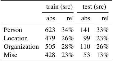
Another aspect that might pose a potential problem to MT is the occurrence of words that were only ob-served a few times or in very particular contexts, as it is often the case for Named Entities. We used the Stanford NER Tagger (Finkel et al., 2005) to detect words that belong to one of four groups: Person, Lo-cation, Organization and Misc. Each group is repre-sented by a binary feature.

Counts are given in Table 2. The test set has sig-nificantly less support for theMisccategory, possi-bly hinting that this data was taken from a different source or document. To avoid the danger of biasing

train (src) test (src)

abs rel abs rel

Person 623 34% 141 33%

Location 479 26% 99 23%

Organization 505 28% 110 26%

Misc 428 23% 53 13%

Table 2: Distribution of Named Entities. The counts are based on a binary features, i.e. multiple occurrences are treated as a single one.

the classifier we decided not to use theMisc indica-tor in our experiments.

3.3 Backoff Behavior

In related work (Raybaud et al., 2011) the backoff behavior of a 3-gram LM was found to be the most powerful feature for word level QE. We compute for each word the longest seen n-gram (up ton = 4) and take the average length as a feature. N-grams at the beginning of a sentence are extended with<s> tokens to avoid penalizing short sentences. This is done on both the source and target side.

3.4 Discriminative Word Lexicon

Following the approach of Mauser et al. (2009) we train log-linear binary classifiers that directly model

p(e|f₁J)for each worde∈eI₁:

p(e|f₁J) = exp

P

f∈fJ

1 λe,f

1 +exp

P

f∈fJ

1 λe,f

(1)

where λe,f are the trained model weights. Please note that this introduces a global dependence on the source sentence so that every source word may influ-ence the choice of all words ineI₁ as opposed to the local dependencies found in the underlying phrase-based MT system.

Assuming independence among the words in the translated sentence we could compute the probabil-ity of the sentence pair as:

p(eI₁|f₁J) = Y

e∈eI

1

p(e|f₁J)· Y

e /∈eI

1

1−p(e|f₁J) . (2)

source resumption of the session target reanudaci´on del per´ıodo de sesiones

Table 3: Example entry of filtered training corpus.

that do not appear in the sentence at hand. We there-fore focus on the observed words and use the geo-metric mean of their individual probabilities:

xDWL(f1J, eI1) =



 Y

e∈eI

1

p(e|f₁J)





1/I

. (3)

We also compute the probability of the lowest scoring word as an additional feature:

xDWLmin(f1J, eI1) = min

e∈eI

1

p(e|f₁J). (4)

3.5 Neural Networks

We seek to directly predict the words in eI₁ using a neural network. In order to do so, both source and target sentence are encoded as high dimensional vectors in which positive entries mark the occur-rence of words. This representation is commonly referred to as thevector space modeland has been successfully used for information retrieval.

The dimension of the vector representation is de-termined by the respective sizes of the source and target vocabulary. Without further pre-processing we would need to learn a mapping from a 90k (|Vf|) to a 170k (|Ve|) dimensional space. Even though our implementation is specifically tailored to exploit the sparsity of the data, such high dimensionality makes training prohibitively expensive.

Two approaches to reduce dimensionality are ex-plored in this work. First, we simply remove all words that never occur in the QE data of 2,254 sen-tences from the corpus leaving 8,365 input and 9,000 output nodes. This reduces the estimated training time from 11 days to less than 6 hours per iteration1. Standard stochastic gradient decent on a three-layer feed-forward network is used.

As shown in Table 3 the filtering can lead to arti-facts in which case an erroneous mapping is learned. Moreover the filtering approach does not scale well as the QE corpus and thereby the vocabulary grows.

1

using a 2.66 GHz Intel Xeon and 2 threads

Our second approach to reduce dimensionality uses thehashing trick (Weinberger et al., 2009): a hash function is applied to each word and the sen-tence is represented by the hashed values which are again transformed using vector space model as above. The dimensionality reduction is due to the fact that there are less possible hash values than words in the vocabulary. To reduce the loss of infor-mation due to collisions, several different hash func-tions are used. The resulting vector representation closely resembles a Bloom Filter (Bloom, 1970).

This approach scales well but introduces two new parameters: the number of hash functions to use and the dimensionality of the resulting space. In our experiments we have used SHA-1 hashes with three different salts of which we used the first 12 bits, thereby mapping the sentences into a 4096-dimensional space.

The results presented in Section 4 based on net-works with 500 hidden nodes which were trained for at least 10 iterations. The networks are not trained until convergence due to time constraints; additional training iterations will likely result in better per-formance. Experiments using 250 or 1000 hidden nodes showed very similar results.

After the models are trained we compare the pre-dicted and the observed target vectors and derive two features: (i) the euclidean distance, denoted as NNdist and HNNdist for the filtered and hashed ver-sions respectively and (ii) the geometric mean of those dimensions where we expect a positive value, denoted as NNprop+ and HNNprob+ in Table 5.

3.6 Edit Distance

source corpus “ ” "

europarl-nc 37 227 25,637

train 0 0 641

test 78 76 100

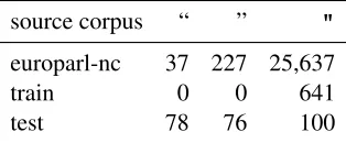
Table 4: Counts of different quotation mark characters.

4 Experiments

In this work we focus on the prediction of human assessment of translation quality, i.e. the regression task of the WMT12 QE shared task. Our submission for the ranking task is derived from the order implied by the predicted scores without further re-ranking.

In general our efforts were directed towards fea-ture engineering and not to the machine learning as-pects. Therefore, we apply a standard pipeline and use neural networks for regression. All parameter tuning is performed using 5-fold cross validation on the baseline set of 17 features as provided by the or-ganizers.

4.1 Preprocessing and Analysis

To avoid including our own judgment, no more than the first ten lines of the test data were visually in-spected in order to ensure that the training and test data was preprocessed in the same manner. Further-more, the distribution of individual characters was investigated. As shown in Table 4, the test data dif-fers from the training corpus in treatment of quo-tation marks. Hence, we replaced all typographi-cal quotation marks ( “, ” ) with the standard double quote symbol (").

Prior to computation of the features described in Subsections 3.3, 3.4 and 3.5 all numbers are re-placed with a special$numbertoken.

Baseline features are used without further scal-ing; experiments where all features were scaled to the[0,1]range showed a drop in accuracy.

While we implemented the training ourselves for the features presented in Subsection 3.5, the open source neural network library FANN2 is used for all experiments in this section. As the performance of individual classifiers shows a high variance, pre-sumably due to local minima, all experiments are conducted using ensembles on500networks trained

2

http://leenissen.dk/fann/wp/

Feature (Section) MAE RMSE |PCC|

BACKOFF (3.3) 0.0 0.0

INDICATORS (3.1) +0.5 +0.7

NER (3.2) +0.5 +0.4

DWLmin (3.4) −0.1 −0.1 0.19

DWL (3.4) 0.0 −0.1 0.36

EDIT (3.6) - tgt words 0.0 0.0 0.32

EDIT (3.6) - tgt chars −0.1 0.0 0.27

EDIT (3.6) - src words 0.0 0.0 0.36

EDIT (3.6) - src chars +0.2 +0.1 0.37

NNdist (3.5) 0.0 0.0 0.35

NNprob+ (3.5) +0.1 +0.2 0.35

HNNdist (3.5) 0.0 0.0 0.37

HNNprob+ (3.5) +0.1 +0.1 0.35

Table 5: Analysis of individual features using 5-fold cross-validation. Positive values indicate improvement over a baseline of MAE57.7%and RMSE72.7%; e.g. including the DWL feature actually worsens RMSE from

72.7%to72.8%.

The last column gives the Pearson correlation coefficient between the feature and the score if the feature is a single column. This information was not used in feature selec-tion as it is not based on cross validaselec-tion.

with random initialization. Their consensus is com-puted as the average of the individual predictions.

4.2 Feature Evaluation

To evaluate the contribution of individual features, each feature is tested in conjunction with all base-line features, using the parameters that were opti-mized on the baseline set. This slightly favors the baseline features but we still expect that expressive additional features lead to a noticeable performance gain. The results are detailed in Table 5. In addi-tion to the main evaluaaddi-tion metrics, mean average error (MAE) and root mean squared error (RMSE), we report the Pearson correlation coefficient (PCC) as a measure of predictive strength of a single fea-ture. Because features are not used alone this does not directly translate into overall performance. Still, it can be observed that our proposed features show good correlation to the target variable. For compari-son, among the baseline features only 2 of 17 reach a PCC of over0.3.

for the translation engine show good performance. In particular binary markers of named entities and and the indicator features introduced in Subsection 3.1 perform well. Further experiments with the latter show their contribution to the systems performance can be attributed to a single feature: the indicator of the genitive case, i.e. occurrences of’sors’.

Testing more combinations of simple and com-plex features may lead to improvements at the risk of over-fitting on the cross validation setup. As a simple remedy several feature sets were created at random, always combining all baseline features and several new features presented in this paper. Averag-ing of the individual results of all sets that performed better than the baseline resulted in our submission.

4.3 Results and Discussion

Of all the features detailed only a few lead to a con-siderable improvement. This is also reflected by our results on the test data which are nearly indistin-guishable from the performance of the baseline sys-tem. While this is disappointing, our more complex features introduce a number of free parameters and further experimentation will be needed to conclu-sively assess their usefulness. In particular, features based on neural networks can be further optimized and tested in other settings.

Even though the machine learning aspects of this task are not the focus of this work we are confident that the proposed setup is sound and can be reused in further evaluations.

5 Conclusion

We described a number of new features that can be used to predict human judgment of translation qual-ity. Results suggest pointing out sentences that are hard to translate, e.g. because they are too complex, is a promising approach.

We presented a detailed evaluation of the utility of individual features and a solid baseline setup for further experimentation. The system, based on an ensemble of neural networks, is insensitive to pa-rameter settings and yields competitive results.

Our new features can potentially be applied for a multitude of applications and may deliver insights into the fundamental problems that cause translation errors, thus aiding the progress in MT research.

Acknowledgments

This work was supported by the MateCAT project, which is funded by the EC under the7thFramework Programme.

References

Arendse Bernth and Claudia Gdaniec. 2001. Mtranslata-bility. Machine Translation, 16(3):175–218, Septem-ber.

John Blatz, Erin Fitzgerald, George Foster, Simona Gan-drabur, Cyril Goutte, Alex Kulesza, Alberto Sanchis, and Nicola Ueffing. 2004. Confidence estimation for machine translation. InProceedings of Coling 2004, pages 315–321, Geneva, Switzerland, August. Burton H. Bloom. 1970. Space/time trade-offs in hash

coding with allowable errors. Communications of the ACM, 13(7):422–426, July.

Peter F. Brown, Stephen A. Della Pietra, Vincent J. Della Pietra, and Robert L. Mercer. 1993. The mathematics of statistical machine translation: Parameter estima-tion. Computational Linguistics, 19(2):263–312. Jenny Rose Finkel, Trond Grenager, and Christopher

Manning. 2005. Incorporating non-local information into information extraction systems by gibbs sampling. InProceedings of the 43rd Annual Meeting on Associ-ation for ComputAssoci-ational Linguistics, ACL 2005, pages 363–370, Stroudsburg, PA, USA.

Arne Mauser, Saˇsa Hasan, and Hermann Ney. 2009. Ex-tending statistical machine translation with discrimi-native and trigger-based lexicon models. In Confer-ence on Empirical Methods in Natural Language Pro-cessing, pages 210–217, Singapore, August.

Sylvain Raybaud, David Langlois, and Kamel Sma¨ıli. 2011. ”this sentence is wrong.” detecting errors in machine-translated sentences. Machine Translation, 25(1):1–34, March.

Lucia Specia, Nicola Cancedda, Marc Dymetman, Marco Turchi, and Nello Cristianini. 2009. Estimating the sentence-level quality of machine translation sys-tems. InProceedings of the 13th Annual Conference of the European Association for Machine Translation, EAMT-2009, pages 28–35, Barcelona, Spain, May. Nicola Ueffing, Klaus Macherey, and Hermann Ney.

2003. Confidence measures for statistical machine translation. In Machine Translation Summit, pages 394–401, New Orleans, LA, September.

Kilian Q. Weinberger, Anirban Dasgupta, John Langford, Alexander J. Smola, and Josh Attenberg. 2009. Fea-ture hashing for large scale multitask learning. In