Error Estimator Using Higher Order FEM for an Interface Problem

(1)

http://www.scirp.org/journal/am ISSN Online: 2152-7393

ISSN Print: 2152-7385

DOI: 10.4236/am.2017.812127 Dec. 18, 2017 1769 Applied Mathematics

Error Estimator Using Higher Order

FEM for an Interface Problem

Maharavo Randrianarivony

1,2

1_{Simulation Unit, Personal Simulation and Design, Sankt Augustin, Germany}

2_{Address: Pappelweg 7, Zimmer 21, Sankt Augustin 53757, Germany}

Abstract

A higher order finite element method is considered to treat an interface prob-lem. The polynomial degree is allowed to be arbitrary but it is fixed for the FEM-variational formulation. We propose an error estimator which turns out to be efficient and reliable. We demonstrate upper and lower bounds of the error estimator with respect to the exact accuracy. For the transmission prob-lem, the coefficients for the internal and external domains can be highly dis-similar. One major difficulty is the characteristic of the estimator at the inter-face. The a-posteriori error estimates can be computed very efficiently ele-ment by eleele-ment. To corroborate the theoretical analysis, we report on a few numerical results.

Keywords

Estimator, A-Posteriori, Interface, Transmission, Higher Order, FEM, Residual

1. Introduction

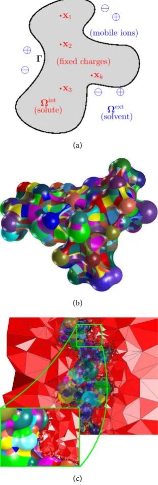
In most aspects of numerical simulation, it is desirable to provide an approximation to an unknown. But it is even more reliable to supply an additional information quantifying how accurate the approximation is. In particular for FEM (Finite Element Method), that additional value is exactly the purpose of the a-posteriori error estimator which is described subsequently. We begin by motivating the transmission problem that is based on the PBE (Poisson-Boltz- mann Equation) for the interaction of solute and solvent media which are respectively denoted by _Ωint _and _Ωext _{. The surface}_Γ_{represents the}

solute-solvent [1] [2] [3] interface which is the molecular surface in the realistic case. The solvent is represented by a continuous dielectric medium while the

How to cite this paper: Randrianarivony, M. (2017) Error Estimator Using Higher Order FEM for an Interface Problem. Ap-plied Mathematics, 8, 1769-1794.

https://doi.org/10.4236/am.2017.812127

Received: November 3, 2017 Accepted: December 15, 2017 Published: December 18, 2017

http://creativecommons.org/licenses/by/4.0/

(2)

DOI: 10.4236/am.2017.812127 1770 Applied Mathematics

solute is located inside the cavity Ωint_{. In the sequel, the whole solute-solvent}

domain is denoted by Ω Ω:= intΩext. The nonlinear PBE [4] admits the next

general expression

( ) ( )

(

)

2

( )

( ) 2

(

)

1 1

4π

e ,

m i

N M

q u C

i i i i

i B i

e

u n q z

k T

β

ε κ − δ

= =

−∇ ⋅ ∇ +

∑

x =

∑

− ∀ ∈

x x x x x x Ω (1)

The charge positions xi are located in the strict interior of the molecular

surface Γ as illustrated in Figure 1(a) and Figure 1(b). The quantities

, , , , , ,

B i i i C

k T z β q n e are constants related to physical parameters while the

(a)

(b)

[image:2.595.296.452.217.695.2]

(c)

(3)

unknown function is the dimensionless electrostatic potential u. The coefficients

( )

ε

x and

κ

( )

x are space-dependent functions related to the dielectric value

and the modified Debye-Hückle parameter. Those coefficients might be discontinuous between Ωint_and Ωext_{but the solution}u_{is required to be}

continuous everywhere. In the case M=2 and under certain assumption on

the parameters, the exponential term becomes a hyperbolic sine. By the Taylor expansion, one has

( )

( ) ( )

3 5

sinh t = +t t 3! + t 5! +. The linear PBE considers

only the first term of the above expansion to obtain

( ) ( )

(

ε u

)

µ

( ) ( )

u f

( )

−∇ ⋅ x ∇ x + x x = x for x∈Ω which will be the purpose of

this paper. We will focus on the FEM treatment of the linearized equation for which we investigate a-posteriori error estimates.

Before presenting our approach, related works and our previous results are in order. Verfürth has compiled a comprehensive study [5] about APEE (a-posteriori error estimator) for which he mainly treats piecewise linear FEM. Many different a-posteriori error estimators have been proposed for the Stokes problem [6] [7] [8] [9] for isotropic grids. In the context of anisotropic meshes

[10] [11] [12], there are a variety of APEEs for Poisson and reaction-diffusion problems [13] [14]. An article [15] by Creusé, Kunert and Nicaise presents a survey on the residual based error estimator on anisotropic grids for the Stokes equation. An interesting APEE for two and three dimensions as well as an anisotropic adaptive mesh refinement are also detailed in [16]. Basically, a-posteriori error estimators permit to evaluate the finite element errors without knowing the exact solution. That feature makes it possible to dynamically identify regions where one should have further refinements if the error there is too large. Therefore, adaptive refinements are mainly based on the quality of a-posteriori error estimators. Our approach in this paper follows the same spirit as the works in [17] [18]. For the Spectral Element Method, we find in [18] an APEE for the hp-case. That is, the mesh size h is allowed to be refined in some regions while the polynomial degrees p are also variable on different elements of the mesh. The hp-case does not require that the polynomial degree or the mesh size are fixed. That has been generalized in [17] to treat hp-FEM [19] for the Poisson problem where corner singularities are allowed. We have presented in

(4)

[26] that is admittedly a very good approach. By inspecting that paper in detail, we realized that a solver in the volume Ω is also needed to construct an artificial fundamental solution. An integral equation solved by BEM is then used by applying that artificial fundamental solution in order to form a kernel. That is, a treatment exclusively on the surface Γ without recourse to a solver in Ω is so far not sufficient. Holst [27] [28] [29] [30] is one of the most prominent specialists of PBE using FEM. His work seems to be extensively based on piecewise linear variational formulation. The Finite Difference Method (FDM) is also widely used in PBE. The main reason does not seem to be attributed to its numerical efficiency but rather to code availability and to reference or comparison purpose (see Section 1.1.2 of [31]). An important component of PBE simulation is the geometric information because exact solutions of PBE are only known for very few simple geometries. Implementing a program for generating an SES (Solvent Excluded Surface) from nuclei coordinates and the Van-der-Waals radii of the atoms is not straightforward because a lot of geometric tasks [32] [33] [34] come into play. It is a long process to start from the nuclei coordinates till obtaining geometric data for computations. We have achieved a geometric task to process nuclei information in order to generate data for BEM as well as a mesh generation [35] from FEM as illustrated in Figure 1(c). Furthermore, a real chemical simulation by using wavelet BEM is described in [25] for the quantum computation. A wavelet BEM simulation using domain decomposition techniques was described in [36] which treats the case of ASM (Additive Schwarz Method). It was utilized as an efficient preconditioner for the wavelet single layer potential which is badly conditioned. A wavelet BEM formulation for computing apparent surface charge is documented in [37] for an interface problem. A simulation for chemical quantum computation using FEM is documented in [38] where we used nanotubes immersed in polymer matrices.

(5)

by the analysis of the a-posteriori error estimator in Section 1. We report on some interesting practical results in the last section.

2. Problem Setting and A-Posteriori Estimators

This section describes the problem formulation, the introduction of the higher order FEM as well as the explicit expressions of the a-posteriori error estimators. We recall also some important results related to polynomial inverse estimates. We consider the transmission PDE:

( )

for

u u f

ε

µ

− int∆ + int = ∈ int

x x x x Ω (2)

( )

for

u u f

ε

µ

− ext∆ + ext = ∈ ext

x x x x Ω (3)

( )

0 0 0

lim u lim u for

→ →

∈ ∈

= ∈

int ext

x x x x

xΩ xΩ

x x x Γ (4)

( ) ( )

( )

0 0

0 0 0 0

lim u , lim u , Q for

ε ε

→ →

∈ ∈

∇ − ∇ = ∈

int ext

x x x x

xΩ xΩ

x n x x n x x x Γ (5)

( )

0 for

u x = x∈∂Ω (6)

where n x

( )

0 designates the normal vector at x0∈Γ pointing outward of = ∂ int

Γ Ω . The load function f :Ω→ and the flux jump Q:Γ→ are

given while the interface Γ and the boundary ∂Ω are polygons in 2  . We consider a mesh h of the entire domain = 

int ext

Ω Ω Ω such that the restrictions of the mesh h in

int

Ω and _Ωext_{are respectively denoted by} h

int_and h

ext_{. The mesh} h

 is composed of triangles admitting the next properties:

 The intersection of two different elements T Ti, j∈h is either empty or a

common node or a complete edge,

 We have the coverings:

, ,

h h h

T T T

∈ ∈ ∈

=



=



=



 int ext

int ext

Ω Ω Ω (7)

 Every node of the interface Γ is also a node of h,

 All edges of the interface Γ are edges of the mesh h.

For a triangle T∈h, we denote

( )

: diameter

( )

sup

{

2, ,

}

h T = T = x y− _R x y∈T (8)

( )

T : supremum of the diameters of all balls contained inT

ρ

= ₍₉₎

( )

T : h T

( ) ( )

T aspect ratio ofT

σ

=

ρ

= (10)

( )

0 T : set of elements of= hsharing a vertex withT

 (11)

( )

: set of elements of sharing a vertex with 1

( )

i T = h T′∈ i− T

  (12)

We use 

( )

T to denote i

( )

T for sufficiently large i. We assume

quasi-uniformity in the sense that there exists a constant ρ >0 0 such that

( )

T 0 , T h

(6)

We define the following mutually disjoint subsets of edges

: set of edges of on the interface

h = h

Γ  _Γ₍₁₄₎

: set of edges of on the boundary ,

h = h ∂

0  Ω ₍₁₅₎

: set of edges of which are not included in ,

h = h

int int _Γ

(16)

: set of edges of which are included neither in nor in .

h = h ∂

ext ext Ω Γ

(17) Note that an edge of h

int_{may have an endpoint in} _Γ_{. Likewise, an edge of} h

ext_{is allowed to have an endpoint in}_Γ_or _∂_Ω_{. We introduce in addition}

the set of all edges

:

h = h  h h  h

 Γ  0 int ext₍₁₈₎

For an edge e∈h, we denote

( )

: length

( )

sup

{

2, ,

}

h e = e = x−y _R x y∈e (19)

( )

e : set of elements of= hhaving as a sidee

 (20)

( )

e : unit normal vector orthogonal to= e

n (21)

The direction of the normal vector n

( )

e is outward Γ if the edge e∈_hΓ while it is pointed toward the exterior of Ω if the edge e∈h

0

. For all other edges in h h

int ext_{, the normal vectors}

( )

e

n are pointed in an arbitrary but

fixed orientation.

For any triangle T, the affine invertible mapping from the unit reference

( )

{

2

}

ˆ : , : 0 1, 0 1, 0 1

T = x= x y ∈R ≤ ≤x ≤ ≤y ≤ + ≤x y (22) onto T is denoted by _{: :}ˆ

T

F T →T in which

( )

(

2

( )

)

( )

1

(

2

( )

)

where det , det

T

Fx=Bx+b B = h T B− = h− T (23) That allows one to derive results on the unit reference triangle _Tˆ_{and to}

carry them over to any element T in the original mesh h. We use the standard

definitions of the Sobolev spaces for 2

( )

_Ω _, 1

( )

_Ω _and 1

( )

0

 Ω . From here onward, we use the usual shorthand XY if there is a constant c such that

X ≤cY in which c is independent on h and p. In addition, X Y amounts to

X  Y X.

We want to consider now the Galerkin variational formulation. Denote the restriction of the solution u to the interface problem in Ωint_and Ωext_by

uint and uext respectively. Due to the Green identity we have

u

u v u v fv v

ε ∇ ⋅∇ +µ = +ε ∂

∂

∫

int

∫

int

∫

int

∫

int int int int int int int int int int

Ω Ω Ω Γ _n (24)

u

u v u v fv v

ε ∇ ⋅∇ +µ = −ε ∂

∂

∫

ext

∫

ext

∫

ext

∫

ext ext ext ext int ext ext ext ext ext

Ω Ω Ω Γ _n (25)

We will denote the piecewise constant function defined on Ω:

( )

if

( )

if

: :

if if

ε µ

 ∈  ∈

=_ =_

∈ ∈

 

int int int int

Ω Ω

ext ext ext ext

x Ω x Ω

x x

(7)

The sum of (24) and (25) for every 1

( )

0

v∈ Ω yields

u u

u v uv fv v

ε

∇ ⋅∇ +

µ

= + _

ε

∂ −

ε

∂ _

∂ ∂

 

∫

Ω

∫

Ω

∫

int int ext ext

Ω Ω Ω Γ _n _n (27)

Taking into account the flux jump (5) in the transmission equation, we have

, , u u

Q=ε ∇u −ε ∇u =ε ∂ −ε ∂

∂ ∂

int ext int int ext ext int ext

n n

n n (28)

The Galerkin weak form is therefore

u v uv fv Qv

ε ∇ ⋅∇ + µ = +

∫

Ω

∫

Ω

∫

Ω Ω Ω Γ (29)

For a fixed polynomial degree p≥1, the finite dimensional space is

( )

{

0

( )

}

: : , in which

h = ∈v vT∈ p ∀ ∈T h

 Ω  Ω   (30)

{

}

: span n m: 0

p = x y ≤ + ≤n m p

 (31)

The discrete Galerkin approximation is to search for uh∈h

( )

Ω such that

( )

,

h h h h h h h h

u v u v fv Qv v

ε ∇ ⋅∇ + µ = + ∀ ∈

∫

Ω

∫

Ω

∫



Ω Ω Ω Γ Ω (32)

Introduce the bilinear form

(

v w,

)

:=

∫

ε ∇ ⋅∇ +v w

∫

µ vw

 Ω Ω

Ω Ω (33)

In order to express the a-posteriori estimators, we assume that the appro- ximated solution uh on the current discretization h is available and we

consider a parameter

α

∈

[ ]

0,1 . The 1D-weight on eˆ=

[ ]

0,1 and the

2D-weight on _Tˆ_{are respectively}

( ) (

)

ˆ

( )

(

)

ˆ 1 and distance , ˆ

e t t t T T

ω = − ω x _ x∂ (34)

For a general edge e and triangle T, transformations from the reference elements are used to define ωe and ωT. For an interior element

int

h

T

∈



,

the estimator is defined as

( )

(

)

2_{( )}

2

2 2

2

,T : 2 T h h T

T

h T

f u u

p

α α

ηint = +εint∆ int−µint int ω

 (35)

where fT designates the 2

( )

T -projection of the load function f onto the

element T. The expression for an exterior element T∈ h ext

 is similar:

( )

(

)

2_{( )}

2

2 ₂

,T : 2 T h h T

T

h T

f u u

p

α α

ηext = +εext∆ ext−µext ext ω

 (36)

For an interface edge e∈h

Γ_{, one introduces}

( )

2 2

2 ₂

, : 2

h h

e e e

e

h e u u

Q

p e e

α α

η = _ −ε ∂ +ε ∂ _ω

∂ ∂

 

int ext

Γ int ext

n n



(37)

where Qe is the 2

( )

e -projection of the flux jump Q onto the edge e. The

estimator for an interior edge e∈h int

(8)

( )

2

2 ₂

, :

2

h

e e

e

h e u

p e

α α

η = ε ∂ ω

∂

 

 

  

int

int int

n (38)

where

 

t stands for the jump of t when evaluated from the two elements incident upon e. The orientation of the jump is irrelevant because one takes its square in the 2_{-norm. The estimator corresponding to an exterior edge}

h

e∈ext is

( )

2

2 2

2 , :

2

h

e e

e

h e u

p e

α α

η = ε ∂ ω

∂

 

 

  

ext

ext ext

n (39)

Since one needs computable local estimators for an element-by-element computation, an interior element T∈h

int

is introduced

( ) ( )

2 2

( )

2

( )

2

, , , ,

, ,

:

h h

T T e e

e T e e T e

α α α α

η η η η

⊂∂ ∈ ⊂∂ ∈

= +

∑

+

∑

int Γ

loc int int Γ ₍₄₀₎

Likewise, for an exterior element T∈h

ext_{, the local estimator reads:}

( ) ( )

2 2

( )

2

( )

2

, , , ,

, ,

:

h h

T T e e

e T e e T e

α α α α

η η η η

⊂∂ ∈ ⊂∂ ∈

= +

∑

+

∑

ext Γ

loc ext ext Γ ₍₄₁₎

The local estimators add up to the global estimator:

( )

2 2

,

:

h

T T

α α

η η

∈

=

∑



loc (42)

One has the following polynomial inverse estimates and extension properties. The descriptions of the next lemmas are found in [17] [19] [39] [40] [41] [42].

Lemma 1. Given

α β

, suchthat − < <1

α β

andsome

δ

∈

[ ]

0,1 . Forevery

univariate polynomial πp of degree p≥1 on the 1D reference element

[ ]

ˆ 0,1

e= , onehas

( )

2

( )

2

1 ₂ 1

ˆ 1 ˆ

0ωe t πp′ t  dt≤C p 0ωe t πp t  dt

∫

(43)

( )

2 ( )

( )

2

1 ₂ 1

ˆ 2 ˆ

0 e t p t dt C p 0 e t p t dt β α

α β

ω _π _ _≤ − ω _π _

   

∫

(44)

( )

2 ( )

( )

2

1 ₂ _{2 2} 1

ˆ 3 ˆ

0 e t p t dt C p 0 e t p t dt δ

δ δ

ω _π_′ _ _≤ − ω _π _

   

∫

(45)

On the 2D reference element (22), one has for every bivariate polynomial πp

of degree p≥1

( )

2

( )

2

ˆ 1 ˆ

ˆ T , p , d d ˆ T , p , d d

T

ω

x y ∇

π

x y x y≤C p T

ω

x y 

π

x y  x y

∫

(46)

( )

2 ₂( )

( )

2

ˆ 2 ˆ

ˆ T , p , d d ˆ T , p , d d

T x y x y x y C p T x y x y x y

β α

α β

ω

_

π

_ _≤ −

ω

_

π

_

   

∫

(47)

( )

2 _{2 2}( )

( )

2

ˆ 3 ˆ

ˆ T , p , d d ˆ T , p , d d

T x y x y x y C p T x y x y x y

δ

δ δ

ω

_∇

π

_≤ −

ω

_

π

_

 

∫

(48)

The constants are C1=C1

(

α β

,

)

, C2=C2

(

α β

,

)

, C3=C3

( )

δ

which do not

depend on p.

Lemma 2. Consideraunivariatepolynomial π ofdegree p≥1 definedon

theunit referenceinterval eˆ=

[ ]

0,1 andaparameter 0 <

γ

≤1. Thereexistsa

bivariate extension 1

( )

_ˆ

(9)

suchthatithasthenextpropertiesw.r.t. theweight eˆ α

ω

:

( )

ˆ ˆ

ˆ e and \ˆ 0

e T e

v =πωα v _∂ ≡ (49)

( )

2 2

2

2 2

ˆ

ˆ e _ˆ

T e

v_ ≤C

α γ πω

α

 (50)

( )

( ) ( )

2 2

2

2 2 2 1 2

ˆ

ˆ e _ˆ

T e

v C

α γ

 p −α

γ

− 

πω

α

∇ _ ≤ _ + _

 (51)

3. Investigation of the Estimators

Theorem 1. Let e be an interface edge in h

Γ_{. Define for the weight}

exponent α:

( )

: h h

e e e

u u

Q

e e

α σ =_ −ε ∂ +ε ∂ _ω

∂ ∂

 

int ext int ext

n n (52)

We have for any γ_{as in (50) and (51) the next estimate using the patch}

( )

e

 : ( ) _{( )}

{

( )

(

( )

)

( )

}

(

)

( ) 2 2 1 2 2 2

2 2 1

2 1

T T

e e _e h h _T

T e

h T

h T e e e

f u u h T

u u p

h T

u u h T Q Q

α

σ ω ε µ γ

γ γ γ ω − ∈ − − ≤ + ∆ − + − + + − + −

∑

      (53)

Under the assumption that 2

h ≤Cp, we have the following bound:

( ) ( ) ( )

( )

( ) (

)

_{( )} 1 2 2 , , 2 2

e p h T T T

T e T e

e e _e

h T

C u u C f f

p h e

Q Q p

α γ γ

α η ω ∈ ∈ ≤ − + − + −

∑

Γ      (54)

Proof. Let Te ∈h int int _and

e h

Text∈ext_{be the two elements which are}

incident upon e. Designate by

σ

e the extension as in (49) of the polynomial

( )

: h h

p e

u u

Q

e e

π

= −

ε

∂ +

ε

∂

∂ ∂

int ext int ext

n n (55)

over the whole patch 

( )

e =Te Te

int ext_{such that we have the restriction}



( )

e p e e

e

α

σ =π ω =σ _{and such that we have the boundary value}

( )



( ) 0

e e

σ

∂ = .

An application of the Green identity, which describes the partial integration of a function with respect to a domain and its boundary, on Te

int

and Te ext yields

(

)

 

( )

 e e e e T h e e

T e T

u u

u

u u

e

ε µ σ

ε σ ε µ σ

− ∆ + ∂ = ∇ ⋅∇ − + ∂

∫

int int int

int int int int

int

int int int int int

n (56)

(

)

 

( )

 e e e e T h e e

T e T

u u

u

u u

e

ε µ σ

ε σ ε µ σ

− ∆ + ∂ = ∇ ⋅∇ + + ∂

∫

ext ext ext

ext ext ext ext

ext

ext ext ext ext ext

n

(10)

Introduce the expressions:

( )

: h h

e

u u

R Q

e e

ε ∂ ε ∂

= − +

∂ ∂

int ext

n n (58)

 

( )



( )



: h h

e e e e e

e e e e

u u

a R Q

e e

σ σ ε ∂ σ ε ∂ σ

= = − +

∂ ∂

∫

int

∫

int ext

∫

ext

n n (59)

( )

e

( )

e

( )

h e

( )

h e

e e e e

u u

e e e e

ε

∂

σ

ε

∂

σ

ε

∂

σ

ε

∂

σ

= − − +

∂ ∂ ∂ ∂

∫

int

∫

ext

∫

int

∫

ext

int ext int ext

n n n n (60)

Apply now (56) and (57) to the last identity in order to obtain a=b where

(

)



(

)



(

)



(

)



(

)



(

)

 : e e e e e e

h h e h h e

T T

h e h e

T T

h e h e

T T

b f u u f u u

u u u u

ε µ σ ε µ σ

ε σ ε σ

µ σ µ σ

= − + ∆ − − + ∆ − + ∇ − ⋅∇ + ∇ − ⋅∇ + − + −

∫

int ext int ext int ext

int int int int ext ext ext ext

int int int ext ext ext

(61)

By adding

∫

_e

(

Qe−Q

)

σe on both sides of a=b, one has on the one hand

(

)



( )



: h h

e e e e

e e

u u

A a Q Q Q

e e

σ  ε ∂ ε ∂ σ

= + − = _ − + _

∂ ∂

 

∫

int int ext ext

n n (62)

( )

2 h h e e e u u Q e e α

ε ε ω

 ∂ ∂ 

= _ − + _

∂ ∂

 

∫

int int ext ext

n n (63)

( )

2

h h

e e e

e

u u

Q

e e

α α

ε ε ω ω−

 ∂ ∂  

 

= _ − _∂ + _∂ _ 

  

 

∫

int int ext ext

n n (64)

( )

2 2

e e e e

e e

α α

σ ω

−

σ ω

−

=

∫

=

 (65)

On the other hand, one has

(

)



(

)



(

)



(

)



(

)



(

)



(

)



(

)

2 2

e

e e

e

e e h h e

e T

h h e h e

T T

h e h e

T T

h e e e e e

T e

B b Q Q f u u

f u u u u

u u u u

u u Q Q α α

σ ε µ σ

ε µ σ ε σ

ε σ µ σ

ε σ ω σ ω−

= + − = − + ∆ − − + ∆ − + ∇ − ⋅∇ + ∇ − ⋅∇ + − + − + −

∫

int ext int ext int ext

int int int int ext ext ext ext int int int ext ext ext int int int ext ext ext

(66)

Hence, we deduce

( )



( )



( )



( )



( )



( )



( )

(

)

_{( )} 2 2 2 2

1 1 1 1

2 2 2 2

2

e e

e e e e

h h _T e

T

h h _T e

T

h _T e h _T e

T T

h _T e h _T e

T T

e e _e

B f u u

f u u

u u u u

Q Q α

ε µ σ

σ σ σ σ ω σ + ∆ − + + ∆ − + − + − + − + − + − int int ext ext

int int ext ext

int int int int

ext ext ext ext

int int ext ext

               ( ) 2 2 e e e α ω−  (67)

(11)

(51), one has



( )

2( )

2

2 ₂ 2

e

e e e e

e

T h T

α

σ γ σ ω−

  int 

int (68)



( )

2( )

2

2 ₂ 2

e

e e e e _e

T h T

α

σ γ σ ω−

  ext 

ext ₍₆₉₎



( )

(

( )

)

( )

1

2

2 1 _{2 2} ₁ ₂ 2

e

e e e _e

T

e

p h T

α α

σ

γ

− ₊

γ

−

σ ω

−



 int  int (70)



( )

(

( )

)

( )

1

2

2 1 _{2 2} ₁ ₂ 2

e

e e e _e

T

e

p h T

α α

σ

γ

− ₊

γ

−

σ ω

−



 ext  ext (71)

A combination of (68)-(71) with the expression of

B

yields

( )

{

( )

( ) ( )

( )

(

( )

)

_{( )} ( )

( )

}

(

)

_{( )} _{( )} 2 2 1 ₂ 2 2 2 2 2

2 2 1 2

2

2 2

1

T T

h h _T e e _e

T e

h T e e _e

h T e e e

e e _e e e _e

B f u u h T

u u p

h T

u u h T

Q Q

α

α α

α

α α

ε µ γ σ ω

γ γ σ ω

γ σ ω

ω σ ω

− ∈ − − − − − + ∆ − + − + + − + −

∑

_ _         (72)

From the equality of A and B, one obtains for the interface edge e∈h Γ_: ( ) _{( )}

{

( )

(

( )

)

( )

}

(

)

( ) 2 2 1 2 2 2

2 2 1

2 1

T T

e e _e h h _T

T e

h T

h T e e e

f u u h T

u u p

h T

u u h T Q Q

α

σ ω ε µ γ

γ γ γ ω − ∈ − − + ∆ − + − + + − + −

∑

       (73)

Consequently, from (52) and the definition (37) of the interface estimator

,e

α

η

Γ _{, one obtains for each fixed polynomial degree} 1

p≥ :

( )

{

( )

(

( )

)

( )

}

(

)

( ) 2 1 2 2 2 2 ,

2 2 2 1

2

2 2

2

1

T T

e h h _T

T e

h T

h T e e e

p

f u u h T

h e

u u p

h T

u u h T Q Q

α

η ε µ γ

γ γ γ ω ∈ − − + ∆ − + − + + − + −

∑

_      Γ (74)

By inserting fT in the last right hand side and by multiplying with

( ) ( )

2

h e p , one deduces

( )

( ) ( ) ( )

( )

( ) (

)

( ) 2 1 2 2 2 2 2 2 , 2 2 2 1

2 2

2

2 2

T T

e T h h _T

T e

h T T T

h T e e e

h T

f u u

p

h T p

u u f f

p p

h T h e

u u Q Q

p p

α

η γ ε µ

(12)

Combine with the estimation of the local residual to obtain:

( )

( ) ( ) ( )

( )

( ) (

)

( ) 1 2 1 2 2 2

2 4 2

2 ₂ ₂

, 2

2 2 2 1

2 2

2

2 2

e h T T T

T e

h T T T

h T e e e

h T p h T

u u f f

p h T p

h T p

u u f f

p p

h T h e

u u Q Q

p p

α

η γ γ

γ γ γ γ ω ∈ − −  ₋ ₊ ₋    ₊  +_ _ − + −    + − _+ − 

∑

        Γ (76)

By regrouping the terms, one obtains

( )

( ) ( ) ( )

( )

( ) (

)

_{( )} 1 2 2 2

2 2 1

2 ₃ 2

,

2 2

e h T

T e

h T T T

e e _e

p

p u u

p

h T h T

u u f f

p p h e Q Q p α α α γ γ η γ γ γ ω − − ∈  ₊   ₊ ₋         + − + − _  + −

∑

      Γ (77)

Then, for the local load oscillation 2₂_{( )}

T T

f − f _ and the local weighted flux oscillation

(

)

_{( )}

2

2 2

e e _e

Q −Q ωα

 one has

( ) ( )

( )

( ) ( )

( )

( ) (

)

( ) 1 2 2 2 2 2 1 3

,

2 2

e h T

T e

T T e e e

T e

h T p

p u u

p p

h T h e

f f Q Q

p p α α α γ γ

η γ γ

γ _ω − − ∈ ∈ + + + − + − + −

∑

      Γ (78)

By using the assumption 2

h ≤Cp, one concludes the last estimate in the theorem.

Theorem 2. Let e be an internal edge in h int₍

resp. an external edge in

h ext

). Undertheassumptionthat 2

h ≤Cp, wehavethefollowingbound:

( ) ( ) ( )

( )

( ) (

)

_{( )} 1 2 2 , , 2 2

e p h T T T

T e T e

e e

e

h T

C u u C f f

p h e

Q Q p

α γ γ

α η ω ∈ ∈ ≤ − + − + −

∑



∑

    int (79) and respectively ( ) ( ) ( )

( )

( ) (

)

_{( )} 1 2 2 , , 2 2

e p h T T T

T e T e

e e _e

h T

C u u C f f

p h e

Q Q p

α γ γ

α η ω ∈ ∈ ≤ − + − + −

∑



∑

    ext (80)

Proof. Define

( )

: h resp. : h

e e e e

u u

e e

α α

σ =ε ∂ ω _ σ =ε ∂ ω _

∂ _ ∂ _                     int ext

int int ext ext

n n (81)

(13)

Theorem 3. Letthedomainoscillationbe:

( ) 2 2 osc : h T T T f f ∈ =

∑

− _ 

Ω ₍₈₂₎

and the interface oscillation be:

( ) 2 2 osc : h e e e Q Q ∈ =

∑

− _ Γ

Γ ₍₈₃₎

The next estimate holds for the weighted error estimator

( )

(

)

( )

1

2 2 2

2 2 2 2

, osc osc

h

h T

T

u u pα

η

α h p hp

∈     − ≤  + +   

∑

  

loc Ω Γ

Ω (84)

Proof. Due to (29), one has for I:=

(

u u w− h,

)

from the bilinear form (33)

(

)

(

)

h h h h h T T T h h h T T T u

I fw Qw u u w w

u

u u w w

ε µ ε

∂ ∈ ∂ ∈  ∂  = + −  − ∆ + +  ∂    ∂  −  − ∆ + +  ∂  

∑

∫

∑ ∫

∫

  int ext ext

int int int int int

Ω Γ

ext

ext ext ext ext ext

n n (85)

(

)

(

)

h h h h h

T T T

T

h

T T T

T

u

I Qw fw u u w w

u

fw v v w w

ε µ ε

∂ ∈ ∂ ∈ ∂   = +  + ∆ − − _∂    ∂   + _ + ∆ − − _ ∂  

∑

∫

∑ ∫

∫

  int ext

int int int int int Γ

ext ext ext ext ext

n

(86)

Every side of ∂T is represented as an edge of h which is categorized in h

Γ_, h 0_,

h int_,

h

ext_{. As a consequence,}

(

)

{

}

(

)

{

}

h h h h T T T T

I f u u w

f v v w A A A A

ε µ ε µ ∈ ∈ = + ∆ − + + ∆ − + + + +

∑ ∫

  int ext

int int int int

ext ext ext ext int ext 0 Γ (87)

:= , : h h h h e e e e u u

A

ε

w A

ε

w

∈ ∈

∂ ₌ ∂

∂ ∂

∑

∫

_ _

∑

∫

_ _

   

int ext

int int ext ext

n n (88)

: , :

h h

h h h

e e

u u u

A

ε

w A Q

ε

w

∈ ∈   ∂ ∂ ∂   = _ _ = −_ − _ ∂ ∂ ∂   _ _

∑

∫

∑

∫

0 Γ

int ext

0 ext Γ int ext

n n n (89)

where A0≡0 because w_∂_Ω=0. Therefore,

( ) ( )

{

}

( ) ( )

{

}

( ) ( ) ( ) ( ) ( ) ( ) 2 2 2 2 2 2 2 2 2 2 h h h h h

h h T T

T T T T h h e e

e e e e

h h

e

e _e

I f u u w

f v v w

u u w w u u Q w ε µ ε µ ε ε ε ε ∈ ∈ ∈ ∈ ∈ ≤ + ∆ − + + ∆ − ∂ ∂ + + ∂ ∂ ∂ ∂ + − − ∂ ∂

∑

                              _ int ext int ext Γ

int int int int

ext ext ext ext

(14)

In particular, for w=

(

u u− h

)

−Ih

(

u u− h

)

where Ih is the Clément

interpolant in [17] [19]. Since 

(

u−u Ih, h

(

u−uh

)

=0, one has

(

)

(

u−u uh, −uh−Ih u−uh

)

=

(

u−u uh, −uh

)

  . ( )

{

( )

(

)

(

)

( )

}

( )

(

)

(

)

( )

{

}

( )

(

)

(

)

_{( )} ( )

(

)

(

)

_{( )} 1 2 2 2 2 2 2 2 2 2 h h h h h

h h h _T h h h _T

T

h h h _T

T T

h

h h h _e

e e

h

h h h _e

e e

e

u u f u u u u I u u

f v v u u I u u

u

u u I u u

u

u u I u u

Q ε µ ε µ ε ε ε ∈ ∈ ∈ ∈ ∈ − ≤ + ∆ − − − − + + ∆ − − − − ∂ + − − − ∂ ∂ + − − − ∂ + −

∑

                 _             int ext int ext Γ

int int int int Ω

int ext in n n ( )

(

)

(

)

_{( )} 2 2 h h

h h h _e

e

u u

u u I u u

ε ∂ ∂ + − − − ∂ ∂   int ext t ext n n (91)

Use the interpolation property of the Clément interpolant [17] [19] to obtain

( )

( ) ( ) ( )

( )

( ) ( ) 1 1

2 , 2

h T T h e e

h T h e

v I v v v I v v

p p

− _ ≤ _ _ − _ ≤ _ _ (92)

Deduce therefore the next estimate

( )

( ) ( ( ))

( )

( ) ( ( ))

( )

( ) ( ( ))

( )

( ) ( ( ))

( )

1 1 2 1 2 1 2 1 2 2 h h h h h

h h h T h T

T h T T T h h e e e h h e e e e h T

u u f u u u u

p h T

f v v u u

p

h e u

u u p

h e u

u u p h e Q p ε µ ε µ ε ε ∈ ∈ ∈ ∈ ∈   − ≤  + ∆ − −      +  + ∆ − −    ∂ + − ∂ ∂ + − ∂ + −

∑

                                  int ext int ext Γ

int int int int Ω

int ext n n ( ) ( ( )) 1 2 h h h e e u u u u

ε ∂ +ε ∂ −

∂ ∂    int ext int ext n n (93) ( )

( )

( ) 1 2 2 2 2 2 2 2 2 2 2 2 2 2 2 2 h h h h h

h h h

T T

h h

e e e e

h h

e _e

h T

u u f u u

p h T

f v v

p

h e u h e u

p p

h e u u

Q p ε µ ε µ ε ε ε ε ∈ ∈ ∈ ∈ ∈  − ≤ + ∆ −  + + ∆ − ∂ ∂ + + ∂ ∂  ∂ ∂ + − + _ ∂ ∂

∑

                           int ext int ext Γ

int int int int

Ω

(15)

Deduce the results for the vanishing weight α≡0:

( )

( ) 2 1 2 1 2 2 2 2 2 0, 0, 2

2 2 2

0, 0,

1 2 2 0,

h h h

h

h h

h

h T T T T

T T T

e e e e

e

e e

e h

e

h T

u u f f

p h e Q Q p u u η η η η η ∈ ∈ ∈ ∈ ∈ ∈ ∈  − ≤ − + +  + + + −  + _ − 

∑

           int ext int ext int int ext Ω int ext Γ Ω (95)

Regroup the local terms with respect to the the local edges to obtain

( )

2( )

( )

1 2

2 2

2 2 2

0, 2

h h h

h T T T e e

T T e

h T h e

u u f f Q Q

p p

η

∈ ∈ ∈

− _ ≤

∑

+

∑

− _ +

∑

− _

  Γ

loc

Ω (96)

For non-vanishing weights α≠0, one applies the polynomial inverse esti-

mate (47) to the polynomial

:

p fT uh uh

π

= +

ε

int∆ int−

µ

int int₍₉₇₎

in order to obtain

( )

(

)

( )

2 2

T h h _T T h h T

T

f +ε ∆u −µ u ≤ pα f +ε ∆u −µ u ωα

 

int int int int int int int int (98)

By using the same thing for the external domain, obtain

( )

2 ₂

( )

2 0,T p ,T

α α ηloc ≤ ηloc _.

Hence,

( )

2( )

( )

1 2

2 2

2 2 2 2

, 2

h h

h T T T e e

T T _e

h

h T h e

u u p f f Q Q

p p α α η ∈ ∈ ∈ − _ ≤

∑

+

∑

− _ +

∑

− _   _ loc Ω Γ (99)

Theorem 4. Foranelement T∈h

int_,respectively

h

T∈ext_,introduce_:

(

)

(

)

: , :

T fT uh uh T T fT uh uh T

α α

σint = +εint∆ int−µint int ω σext = +εext∆ ext−µext ext ω ₍₁₀₀₎

One has for a fixed polynomial degree p≥1 the following estimates

( )

(

)

( )

2 1 2

2

2 2

T T _T h _T T T _T

p

u u f f

h T

α

α α

σ ω

− − ₋ ₊ ₋

ω

   

int int int ₍₁₀₁₎

( )

(

)

( )

2 1 2

2

2 2

T T h T T

T T T

p

u u f f

h T

α

α α

σ ω

− − ₋ ₊ ₋

ω

   

ext ext ext ₍₁₀₂₎

Thus, the local expressions

η

α,T int _and

,T

α

η

ext _verify:

( )

( ) (

)

( )

1 2

2

,T p, h _T T T _T

h T

C u u f f

p

α α α

η ≤ − + − ω

 

int int int ₍₁₀₃₎

( )

( ) (

)

( )

1 2

2

,T p, h _T T T _T

h T

C u u f f

p

α α α

η ≤ − + − ω

 

ext ext ext ₍₁₀₄₎

Proof. The following equalities hold:

( )

(

)

2

2 2

T T _T _T fT uh uh T

α α

σ ω− ₌ ₊ε _∆ ₋µ ω

∫



int int int int int ₍₁₀₅₎

(

h h

)

T

(

T

)

T

T f ε u µ u σ T f f σ

(16)

(

)

T T h T

T T T

h T T T

T T

u u u

u f f

ε σ µ σ ε σ

µ σ σ

= ∇ ⋅∇ + − ∇ ⋅∇

− + −

∫

int int int int int int int int int

int int int int (107)

(

)

(

)

(

)

2 2

h T h T

T T

T T T T

T

u u u u

f f α α

ε σ µ σ

ω σ ω−

= ∇ − ⋅∇ + −

+ −

∫

int int int int int int int

int (108)

Consequently, one obtains

( ) 1( ) 1( )

(

)

( ) ( )

2 2 2

T T T u uh T T T fT f T T T T T

α α α

σ ω− ₋ σ ₊ ₋ ω σ ω−



    

int int int int ₍₁₀₉₎

Concerning the estimation of σT _1_{( )}_T

int _{, one has}

( )

{

(

)

}

1

2

T _T _T fT uh uh T

α

σ =

∫

∇ +ε ∆ −µ ω



int int int int int (110)

(

)

(

)

2 2 2 2 2

T T h h

T

T h h T

T

f u u

α

ω ε µ

ε µ ω

≤ ∇ + ∆ −

+ + ∆ − ∇

∫

int int int int int int int int

(111)

For the first term, apply the polynomial inverse estimate (48) to the polynomial

:

p fT uh uh

π

= +

ε

int∆ int−

µ

int int₍₁₁₂₎

and the affine transform _: ˆ

T

F T→T in order to obtain

(

)

2 2(

( )

)

(

)

2 2

2

T T h h T T h h

T T

p

f u u f u u

h T

α

α α

ω

∇ +

ε

∆ −

µ

−

ω

+

ε

∆ −

µ

∫

int int int int 

∫

int int int int ₍₁₁₃₎

As for the second term, split T 2

α

ω

∇ _into

(

)

2

x T

α ω

∂ and

(

)

2

y T

α ω

∂ , use the boundedness of T

α

ω

_{and apply the inverse estimate (47) to the polynomial (112)}

to obtain

(

)

2 2(

( )

)

(

)

2 ₂ 2 2

2

T h h T T h h T

T T

p

f u u f u u

h T

α

α α

ε

µ

ω

−

ε

µ

ω

+ ∆ − ∇ + ∆ −

∫

int int int int 

∫

int int int int ₍₁₁₄₎

A combination of (111), (113) and (114) yields

( ) ( )

( )

(

)

1 2 2 2 2

T _T T h h T

T

p

f u u

h T

α

σ

−

∫

+

ε

∆ −

µ

ω

 

int int int int int ₍₁₁₅₎

( )

{

(

)

}

( )

2( )

2 2 2 2 2 2 2 2 2

T h h T T

T

T T _T

p

f u u

h T p h T α α α α α

ε µ ω ω

σ ω − − − − = + ∆ − =

∫



int int int int

int

(116)

As a consequence, one has

( ) ( )

( )

( ) ( )

(

)

_{( )} _{( )} 1 2 2 2 2 2 2 2 2 2 2

T T _T h _T T T _T

T T _T T T _T

p u u h T f f α α α α α

σ ω σ ω

ω σ ω

− − − − − + −      

int int int int

int

(117)

(17)

( )

(

)

( )

2 1 2

2 2

T T _T h _T T T _T

p

u u f f

h T

α

α α

σ ω

− − ₋ ₊ ₋

ω

   

int int int ₍₁₁₈₎

By using the definition (35) of the interior estimator, one has

( )

_{( )}

2 2

2 ₂ 2

,T 2 T T _T

h T p

α α

η

₌

σ ω

−



int int ₍₁₁₉₎

( )

( ) (

)

( )

1 2

2 2 2

2

2 h _T 2 T T _T

h T p

u u f f

p p

α

ω

−

− + −

 

 int int

(120)

The other estimates are obtained in a similar manner.

4. Practical Results

The computer implementation is performed by a combination of C functions and C++ classes. Some LAPACK and BLAS routines are used sometimes to perform various linear algebraic operations.

4.1. Exact Precision

In this subsection, we concentrate fully on the exact precision for the purpose of obtaining insight and confidence about the accuracy of the results of the computer implementation. That is, we do not consider yet any description of the error estimator ηα. We examine several parameters comprising the polynomial

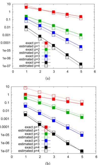
degree and the problem coefficients _εint,εext,µint,µext_. The ε-ratio and the μ-ratio