Simulation of Fluid Structure Interactions by using High Order FEM and SPH

Simulation of Fluid Structure Interactions by using High Order FEM and

SPH

Sebastian Koch∗_{, Sascha Duczek}†_{, Fabian Duvigneau}∗_{and Elmar Woschke}∗ ∗_{Institute of Mechanics}

Otto von Guericke University Magdeburg Universit¨atsplatz 2, 39106 Magdeburg, Germany

e-mail: [email protected], web page: www.ifme.ovgu.de/

†_{School of Civil and Environmental Engineering}

University of New South Wales, Sydney ABSTRACT

The investigation of fluid structure interactions is crucial in many areas of science and technology. This study presents a robust methodology for studying fluid structure interactions, which is characterized by high convergence behavior and is insensitive to distortion and stiffening effects. Therefore, the Smoothed Particle Hydodynamicy is coupled with the high order FEM. After various coupling methods for linear and quadratic elements from the literature have been described, a variant with higher-value approach functions is implemented. The two methods can be meshed independend without loss of accuracy. After successful validation, it is shown that only a few finite elements are necessary to obtain a convergent solution. The presented method is promising especially for thin-walled structures where significantly fewer degrees of freedom are required than for linear elements.

1 Introduction

In many fields of science and engineering, we know that the interaction of fluids with structures has an important effect on the behavior of the overall system. For this reason, effective and robust methods for describing these interactions have been the subject of intensive research activities throughout the last decades. Figure 1 shows three typical applications in which an accurate description of the Fluid Struc-ture Interaction (FSI) is essential for capturing the dynamics of the system. A section of an automatic fluid ball balancing unit of a centrifuge is depicted in Figure 1a. Among other things, the ball position depends on the flow conditions and thus influences the vibration behavior of the system [1]. In Figure 1b components of a turbocharger system such as shaft, turbine and compressor are shown. Additionally, the pressure distribution in the floating ring bearings resulting from the operating condition are indicated. It should be clear that dynamical response of a turbocharger can only be described in a meaningful way by taking the hydrodynamics in the bearings into account [2]. As a third example, in which the considera-tion of FSI is essential, Figure 1c illustrates the sound radiaconsidera-tion caused by the structural vibraconsidera-tions of an engine block. Here, the surrounding fluid (air) has to be considered for the simulation [3].

For the numerical investigation of FSI, various numerical procedures are available and their effectiveness depends on the specific characteristics of the problems that is investigated. An accurate description of the effect induced by the interaction provides an opportunity to estimate the performance of new products already in an early stage of the product development cycle. Thus, the design can be enhanced in order to reach project specific goals. In addition, expensive prototypes are only required for the final testing as well as for validation purposes. Due to the importance of considering FSI in several applications, the overarching goal of this contribution is to develop a robust numerical method which features high rates of convergence.

In this contribution the solid (deformable) structure is described using the finite element method (FEM) which is the dominant method for solving problems in structural dynamics. In order to improve this ap-proach a special focus is placed on using high-order FE shape functions, making this numerical method

insensitive to locking effects and element distortion [5]. An additional advantage are high possibly ex-ponential rates of convergence [6].

The liquid phase is described using the smoothed-particle hydrodynamics (SPH) method, which is a particle-based, meshless Lagrangian method [17]. Possible areas of application are multiphase flows, moving interfaces and problems with large changes in the fluid area. A coupling between SPH and FEM has been successfully realized with linear [7–9] or quadratic [10] FEs and is well-suited for the descrip-tion of fluid structural interacdescrip-tions. The novelty of our approach lies in the coupling of SPH to high order FEs which results in advantages with respect to locking effects and element distortion being of interest when thin-walled structures are investigated.

The performance of the proposed methodology will be evaluated based on a simple academic bench-mark test. As mentioned before due to the coupling of high order FEM and SPH the influence of a fluid phase on the vibrational behavior of a thin walled structure such as an oil pan can be straightforwardly investigated. By using the high order FEM, the thin-walled structures can be described effectively, since these elements are robust against distortion (large aspect ratios). Here, it is observed that the fluid has a significant effect on the dynamic behavior of the structure [3]. This has also a notable effect on the noise emission and is, therefore, of utmost importance for the acoustic properties of the structure.

2 High order finite element method

The basic idea of the FEM is the division of the considered domain in smaller sub-domains, so-called finite elements. The exact solution of the mathematical problem is often approximated by simple poly-nomial ansatz functions, which are defined only within a finite element. In order to obtain a convergent solution, a distinction is frequently made between theh-,p-andhp-versions of the FEM [11, 12]. In the

h-version of the FEM, which is implemented in all commercial FE programs, convergence is achieved through the refinement of the mesh. A mesh refinement can be conducted both globally and locally, i.e. the element dimensionhis reduced until a convergent solution is reached (h → 0). In the case of the p version of the FEM, the element dimensions are kept constant and the polynomial degree pis suc-cessively increased. Commercial FE programs usually have maximally quadratic elements (p ≤ 2). A combination of the two presented methods leads to thehp-FEM which ensures exponential convergence even for singular problems.

In general, it can be stated that higher-order ansatz functions are to be favored, since higher convergence rates (possibly even exponential ones) can be achieved. An additional advantage is their robust behav-ior with respect to locking phenomena and element distortions. As a result, highly accurate results can be achieved even with highly distorted elements [6]. Figure 2 illustrates the benefits of higher order ansatz functions in terms of improved convergence rates. The error is plotted in the energy norm over the number of degrees of freedom of the system in a log-log diagram. For problems that exhibit a smooth solution, the convergence curve for the p-FEM follows an exponential curve, while theh-FEM shows

(a) Ball balancing unit [1] (b) Turbocharger [4] (c) Sound radiation [3] Figure 1: Typical problems with FSI.

Figure 2: Convergence rates of theh-,p-andhp-Version FEM for a two dimensional linear problem with singularities [6].

only algebraic convergence. Even for problems involving singularities, the convergence rate of the

p-version of the FEM is at least twice than of theh-FEM. If theh-refinement is suitably combined with thep-adaptation, an exponential convergence can be achieved even in the case of problems with singular locations. Therefore, the application of higher-order shape functions (p ≥ 3) is recommended in many

cases.

3 Smoothed-particle hydrodynamics

SPH is a numerical method in which the bodies and fluids in the solution area are approximated by a set of particles. In addition to position and velocity, these particles are associated with additional information such as mass, pressure and temperature of the approximated amount of material. SPH is a Lagrangian method and thus the particles move together with the approximated material. The method was presented by Lucy [13] and Gingold & Monaghan [14] for astrophysical investigations and is nowadays widely used for fluid dynamics [15, 16]. The fundamental idea is based on the integral approximation of a quantityAof the fluid particleiunder consideration of the neighboring particles j

Ai(r) =

A(r)W(r₋r_j,h)dr_j, (1)

whereW is the kernel function,hthe kernel length,rthe location anddrja differential volume element. This approximation is exact if the delta function is chosen for the kernel. Hence, the integral given in Eq. (1) can be approximated by a summation over all particlesnwithin the influence area

Ai(r) = n

∑

mjA_ρj j W

(r₋r_j,h_j)_. (2)

A typical set-up of SPH simulations is sketched in Figure 3, where a particlei(red), its neighbor particles (blue), the influence area, which is a multiple of the kernel lengthh(depending on the kernel function) and the kernel function are depicted. The function value indicates the influence of a neighboring particle exerts on the central particle.

An advantage of SPH is that the path of a particle can be traced exactly. In this way, mixing and boundary layers can be effectively described. The treatment of different materials is very simple by introducing different particle properties and the interactions can be implemented in a straightforward fashion. An-other advantage is that only domains that are filled with the material (fluid) need to be discretized and

Influence radius Influence radius Influence radius Influence radius Influence radius Influence radius Influence radius Influence radius Influence radius Influence radius Influence radius Influence radius Influence radius Influence radius Influence radiusInfluence radiusInfluence radius Central particle Kernel function Neighbor particles Neighbor particles Neighbor particles Neighbor particles Neighbor particles Neighbor particles Neighbor particles Neighbor particles Neighbor particles Neighbor particles Neighbor particles Neighbor particles Neighbor particles Neighbor particles Neighbor particles Neighbor particlesNeighbor particles

Figure 3: Central particle with neighbor particles, influence area and kernel function [18]. therefore, no numerical costs are incurred in areas that are not immersed. In Eulerian methods, the entire simulation area has to be meshed and calculations are executed for the whole domain in each time step. A detailed description of the method including its derivation for fluid dynamics can be found in [17]. In this contribution, dynamic boundaries are used [19]. That is to say, particles with the same proper-ties as the fluid particles are placed at the boundaries of the structure. However, these particles have no translational degrees of freedom (fixed at the current position or move along a given path). In this way, a penetration of the boundary is prevented.

4 Fluid Structure Interaction – SPH-FEM coupling

In the following, FSI investigations based on coupling SPH andh-FEM are presented. It has been shown that it is adequate for some studies to consider the solid as a rigid body. A primary example for this case are offshore platforms, interactions of ships and tsunami, where the influence of the rigid body on the wave breaking is investigated [20, 21]. The influence of including elastic bodies was considered and was investigated by different authors. The first publication, which is known to the authors of this paper, is from Attaway [7]. This study showed an SPH-FEM interaction of two identical solid bodies which were pressed against each other. The coupling was realized with a master slave concept. Therefore, the penetration of the slave (SPH) body by the master (FEM) body was prevented using a penalty approach (coupling forces). This coupling was realized for solid-solid interaction, the possibility for FSI was not realized but already mentioned in the article. Another realization of FSI using FEM-SPH coupling was proposed by De Vuyust [22]. In this application, dynamic boundary conditions were used, i.e. in the area of contact SPH particles that coincide with the nodes of a FEM discretization were deployed. The displacement of the FE-Nodes directly translates to a displacement of the corresponding SPH boundary particles. By treating the FE nodes as SPH particles they act as boundary particles and cause a repulsive force as fluid particles approaches. The generated force acts equally on both fluid and solids. In this way, a penetration of the boundary is prevented and additionally the force is transferred from the fluid particles to the elastic body (FE model). The sum of the acting forces is equal to zero according to Newton’s third law. Forces exerted by fluid particles on boundary particles are distributed among the nodes using the element ansatz functions. In Ref. [22] three application examples were discussed, whereby a coupling of fluid and elastic body was not presented. A different type of coupling conditions was introduced by Fourey [9] who uses the fluid pressure for FSI (referred to as pressure coupling). The pressure value at a FE node is calculated from the average of the pressures of the fluid particles that are in the influence area of the FE node. With this method, the mesh size of both variants is independent of each other. The

penetration of the solid by the fluid was prevented using so-called ghost particles. That is to say, the fluid particles are mirrored at the boundary and the new particles are treated like fluid particles, while their movements depend on their parent particles. Another concept, similar to Attaways [7] master-slave coupling, is used by Yang [8]. By using repulsive boundaries, fluid particles get a repulsive force as a function of their wall distance normal to the boundary. This force acts on the FE system in the same size and in the opposite direction. The element ansatz function distributes the force to the nodes of the element involved (penalty coupling).

The possibility to describe both fluid and solid with a SPH approach is also briefly mentioned. Rafiee [23] verified a pure SPH-based methodology and obtained a good agreement compared to previously pub-lished results. This approach will not be discussed in this study, since both the imaging quality of solids in comparison to the FEM is worsened and the numerical complexity increases significantly [24]. FEM is by far the most widely used method for solving partial differential equations and is therefore considered to be a useful supplement to SPH in order to efficiently describe the elastic bodies.

The presented couplings of SPH and FEM from literature uses linear FE elements, but even quadratic elements have already been implemented [10]. Higher ansatz functions have not been considered to the knowledge of the authors. Consequently, the paper at hand is an extension of the current state of the art.

5 High order FE-SPH-Coupling

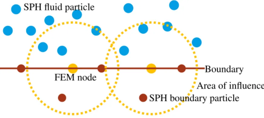
FEM and SPH interact via pressure (nodal forces) respectively force that is exerted by the fluid particles on the FE mesh. This results in displacements of the FE nodes which are transferred to the particles; i.e. SPH provides the loads for the FEM, and the FEM transfers the resulting structural displacements and velocities to the SPH particles. The coupling implemented here is based on the work of Fourey [9]. The pressure at a FE node is determined by the mean value of the particle pressures in its influence domain. In Figure 4 this concept is visualized for a two-dimensional setting. Three fluid particles (blue) are de-tected in the influence area of the left FE-node (orange). The pressure values associated with these fluid particles are averaged and converted into an equivalent nodal load which is achieved by integrating the pressure distribution over the face of an immersed FE. In determining the nodal forces, it is important to accurately approximate the discrete pressure function (given only at the fluid particles). One idea is to interpolate the pressure function using a simple polynomial distribution along the boundary of immersed FEs. Figure 5 shows an example of the distribution of nodal forces for a constant pressure along an element boundary for linear, quadratic and higher-order finite elements. Here, already the non-constant distribution of the force values on the nodes is observed. This results from the computation of energet-ically equivalent nodal loads under consideration of the element ansatz functions. The equivalent nodal forceFeis calculated based on the pressure valuesp(ξ)and the ansatz functionN(ξ)along the surfaceΓ

Fe=

ΓN

T_{(ξ) p(ξ)dΓ. (3)}

De Vuyust [22] used a node-particle dualism creating points that are both SPH boundary particles and FE nodes. That is one suitable option but not necessary, especially when considering the coupling with high order FEM, because the nodal distribution is not equidistant for most variants [25] and therefore, it is recommended to discretize the two systems separately. In order to interpolate the particle movement of a SPH fluid particle, the element ansatz functions are used (note that fluid particles are located at arbitrary positions on the element boundary which do not generally coincide with a FE node). Therefore, the local coordinates ξj of the SPH particle within a FE are determined, at the beginning of the simulation by solving the following non-linear system of equations (inverse mapping)

xSPH,j= n

∑

SPH fluid particle

SPH boundary particleArea of influence

FEM node Boundary

Figure 4: Two rows of boundary particles (brown) that prevent the fluid particles (blue) from penetrating the boundary and FE nodes (orange) with the area of influence, from which the fluid pressures are averaged.

Figure 5: Determination of equivalent node load at a constant pressure distribution at different higher orders p of the ansatz function. From left to right: Element with constant pressure, Linear element, Quadratic element, Cubic element, Quadratic element, Quintic element

with respect to ξj. Where i is the number of FE nodes in an element, Ni is the ansatz function cor-responding to nodei, andxi,j is the global coordinate of the nodeiin the j-dimensional space. Now, the displacement of the SPH particleuSPH can be determined using the displacement resultuof the FE

simulation

uSPH,j= n

∑

Ni(ξj)ui,j. (5)

These determination does not cause loss of accuracy. By using the ansatz functions, the particular dis-palcements are exact in terms of the discretization. In this way, the FEM and SPH systems can be independently discretized. That is to say, different to the approach taken by De Vuyust, it is not nec-essary that SPH particles and FEM nodes are at the same position. This is particularly advantageous because many high order FEM variants do not have an equidistant nodal distribution, which is, however, a prerequisite in the set-up of the initial SPH discretization.

6 Dam break with a rigid obstacle

For the FEM, an in-house developed FE code is used, which also allows different high order approaches [5]. In this contribution, conventional serendipity elements are deployed with an order of p≤4. For the description of the fluid, the open source software SPHysics is used. This code has been utilized in different scientific contexts [26–28] and has there been thoroughly verified and validated.

The well-known example of a dam break and a rigid obstacle is used to demonstrate the FSI with a solid structure. The dimensions can be taken by Figure 6. In Figure 7 the water profile obtained in the experiment (photo and red line), a SPH simulation from literature [23] (green line) and our own implementation in SPHysics are compared. A good agreement between our simulation results and the

b

L 4 L

Rigid obstacle

Elastic obstacle L = 14.6 cm b = 2.4 cm h = 4.8 cm L = 14.6 cm b = 1.2 cm h = 8 cm Rigid or

elastic ostacle Water

column

Wall

Wa

ll

Wa

ll

2 L

L

h

Figure 6: Initial geometry of the water column with a rigid respectively an elastic obstacle [23].

0 s

0.1 s

0.2 s

0.3 s

0.5 s

1.0 s

Figure 7: Comparison of water profile of experimental results (left and red line) with SPH simulations (Rafiee, green line) [23] and SPHysics implementation (blue particles) for a collapsing water column with rigid obstacle.

ones published by Rafiee [23] can be observed. The results at the left and right boundaries of the domain do not seem to be physical as a part of the fluid stays attached to the walls until 0.5 s after the dam break (green line). This effect does not occur in our simulations and is also not observed in the experimental measurements. In [23] the difference was attributed to the neglected air in the simulation. The input values used for this verification example (See Appendix 1) are used for all further investigations.

7 Dam brake with an elastic obstacle

The second example is a typical benchmark test that is often employed to verify FSI applications in the context of SPH. We use a similar geometry as in the previous example but for this simulation it is

assumed that the obstacle is not rigid any more and the dimensions of the obstacle are adjusted. The geometry is depicted in Figure 6. This example was already used by various authors [10, 23, 29, 30], but unfortunately experimental results are not available, at least to the authors’s knowledge. Figure 8 shows the displacement of the upper left point of the obstacle over time, with 240 or 60 quadratic FE elements and 10000 SPH fluid particles, and a comparison with results taken from literature [10, 23]. In [10], Hu also used 60 or 240 FE elements but 5000, 80000 and 180000 fluid particles. He introduced an efficient search algorithm (which is currently not implemented in SPHysics) and therefore was able to deploy this large number of particles. At the beginning the results are comparable with the literature [10, 23, 29, 30], later on there are clear differences. This differences can be attributed to the large deformations that occur in the verification example. To account for the effects of geometrical non-linearity the second

Figure 8: Comparison between numerical results for time history of the displacement of the upper left corner, using 10000 Fluid particles and 60 respectively 240 FEs.

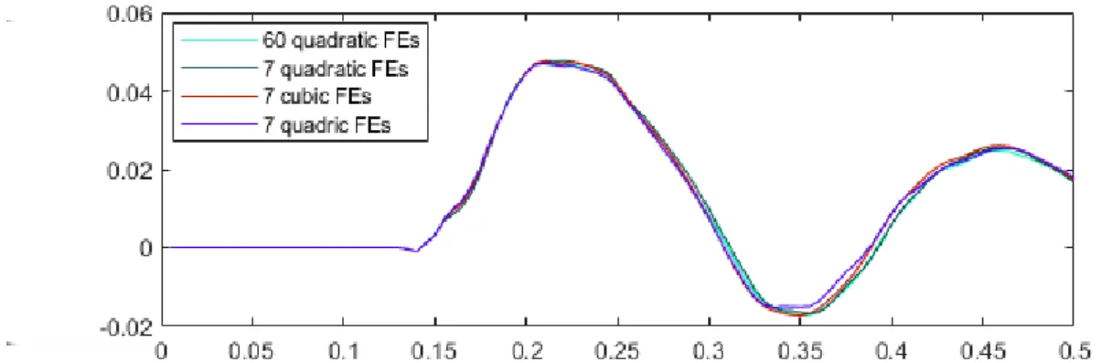
Figure 9: Comparison between numerical results for time history of the displacement of the upper left corner, using 10000 Fluid particles and seven FEs.

Figure 10: Comparison between numerical results for time history of the displacement of the upper left corner, using 10000 Fluid particles and one FE.

Piola-Kirchhoff stress tensor was used in [30]. The FEM program used in this work is based on the linear theory of elasticity which is sufficient to account for the influence of a fluid on the vibration behavior being investigated in forthcoming publications by the authors. This does not constitute a limitation of the proposed approach as geometrically and physically nonlinear behavior can be straightforwardly added to high order FE codes [31]. The deformations at 60 and 240 quadratic elements are similar, so the solution is converged. Subsequently, this solution is to be realized with significantly fewer elements and ansatz functions of different order. Figure 9 shows the displacement of the upper left corner using seven FE ele-ments and different ansatz functions compared to 60 quadratic Eleele-ments. It is good to see that the higher elements are able to describe the vibration behavior of the obstacle. Already seven quadratic elements are sufficient. Despite the large deformations that occur, the results are still in relatively good agreement. In order to clarify the potential of high order FEM, Figure 10 shows the displacement using one FE of different order. It is good to see that a polynomial order of three or higher is sufficient for the vibration analysis. In future studies, validation examples with small deformations are considered to demonstrate the performance of high order FE-SPH coupling.

8 Conclusion

A coupling of SPH and high order FEM was shown and verified, which allows to describe the solid body efficiently using only a few FEs. The insensitivity of high order methods with respect to locking ef-fects and element distortion makes it ideal for the discretization of thin-walled structures. The proposed pressure coupling can be easily implemented in existing codes. Other possible coupling schemes from literature were briefly mentioned but not implemented and validated in the context of high order FEM. Such an implementation is analogous to the one presented in this contribution and is easily possible. In addition to serendipity elements used here, other higher order approaches are conceivable. In further work, different coupling strategies as well as FE ansatz functions will be investigated and evaluated. Furthermore, a three-dimensional variant is to be implemented and experiments to validate the results are performed.

Acknowledge

The presented work is part of the joint project KeM (Kompetenzzentrum eMobility), which is financially supported by the European Union through the European Funds for Regional Development (EFRE) as well as the German State of Saxony-Anhalt (ZS/2018/09/94461). This support is gratefully acknowledged.

[1] L. Spannan, C. Daniel, and E. Woschke. “Experimental study on the velocity dependent drag coefficient and friction in an automatic ball balancer”. In:Technische Mechanik - Scientific Journal for Fundamentals and Applications of Engineering Mechanics37.1 (2017), pp. 180–189.

[2] Christian Daniel, Stefan G¨obel, Steffen Nitzschke, Elmar Woschke, and Jens Strackeljan. “Numer-ical simulation of the dynamic behaviour of turbochargers under consideration of full-floating-ring bearings and ball bearings”. In:11th international conference on vibration problems. Vol. 400. 2013, p. 23.

[3] F. Duvigneau, S. Nitzschke, E. Woschke, and U. Gabbert. “A holistic approach for the vibration and acoustic analysis of combustion engines including hydrodynamic interactions”. In:Archive of applied mechanics : (Ingenieur-Archiv)(2016).

[4] S. Nitzschke, E. Woschke, C. Daniel, and J. Strackeljan. “Simulation von Schwimmbuchsen-lagerungen in Abgasturboladern”. In:Journal of Mechanical Engineering of the National Techni-cal University of Ukraine KPI61.2 (2011), pp. 7–12.

[5] S. Duczek.Higher Order Finite Elements and the Fictitious Domain Concept for Wave Propaga-tion Analysis. VDI Fortschritt-Berichte Reihe 20 Nr. 458, 2014.

[6] A. D¨uster.High Order Finite Elements for Three-Dimensional, Thin Walled Nonlinear Continua. Shaker, 2002.

[17] Joe J Monaghan. “Smoothed particle hydrodynamics”. In: Reports on progress in physics 68.8 (2005), p. 1703.

[7] SW Attaway, MW Heinstein, and JW Swegle. “Coupling of smooth particle hydrodynamics with the finite element method”. In:Nuclear engineering and design150.2-3 (1994), pp. 199–205. [8] Qing Yang, Van Jones, and Leigh McCue. “Free-surface flow interactions with deformable

struc-tures using an SPH–FEM model”. In:Ocean engineering55 (2012), pp. 136–147.

[9] G Fourey, G Oger, D Le Touz´e, and B Alessandrini. “Violent fluid-structure interaction simu-lations using a coupled SPH/FEM method”. In:IOP conference series: materials science and engineering. Vol. 10. 1. IOP Publishing. 2010, p. 012041.

[10] Dean Hu, Ting Long, Yihua Xiao, Xu Han, and Yuantong Gu. “Fluid–structure interaction analysis by coupled FE–SPH model based on a novel searching algorithm”. In: Computer Methods in Applied Mechanics and Engineering276 (2014), pp. 266–286.

[11] B. Szab´o, B. A. Szabo, and I. Babuˇska.Finite element analysis. John Wiley & Sons, 1991. [12] B. Szab´o and I. Babuˇska. Introduction to finite element analysis: formulation, verification and

validation. Vol. 35. John Wiley & Sons, 2011.

[13] Leon B Lucy. “A numerical approach to the testing of the fission hypothesis”. In:The astronomical journal82 (1977), pp. 1013–1024.

[14] R. A. Gingold and J. J. Monaghan. “Smoothed particle hydrodynamics: theory and application to non-spherical stars”. In:Monthly Notices of the Royal Astronomical Society181.3 (1977), pp. 375– 389.

[15] MS Shadloo, G Oger, and D Le Touz´e. “Smoothed particle hydrodynamics method for fluid flows, towards industrial applications: Motivations, current state, and challenges”. In:Computers & Flu-ids136 (2016), pp. 11–34.

[16] Hitoshi Gotoh and Abbas Khayyer. “Current achievements and future perspectives for projection-based particle methods with applications in ocean engineering”. In:Journal of Ocean Engineering and Marine Energy2.3 (2016), pp. 251–278.

[18] R. Sampath, N. Montanari, N. Akinci, S. Prescott, and C. Smith. “Large-scale solitary wave sim-ulation with implicit incompressible SPH”. In:Journal of Ocean Engineering and Marine Energy

2.3 (2016), pp. 313–329.

[19] AJC Crespo, M G´omez-Gesteira, and Robert A Dalrymple. “Boundary conditions generated by dynamic particles in SPH methods”. In:CMC-TECH SCIENCE PRESS-5.3 (2007), p. 173. [20] B. Ataie-Ashtiani and G. Shobeyri. “Numerical simulation of landslide impulsive waves by

incom-pressible smoothed particle hydrodynamics”. In:International Journal for numerical methods in fluids56.2 (2008), pp. 209–232.

[21] Tim Verbrugghe, Jos´e Manuel Dom´ınguez, Alejandro JC Crespo, Corrado Altomare, Vicky Strati-gaki, Peter Troch, and Andreas Kortenhaus. “Coupling methodology for smoothed particle hy-drodynamics modelling of non-linear wave-structure interactions”. In:Coastal Engineering138 (2018), pp. 184–198.

[22] Tom De Vuyst, Rade Vignjevic, and JC Campbell. “Coupling between meshless and finite element methods”. In:International Journal of Impact Engineering31.8 (2005), pp. 1054–1064.

[23] Ashkan Rafiee and Krish P Thiagarajan. “An SPH projection method for simulating fluid-hypoelastic structure interaction”. In:Computer Methods in Applied Mechanics and Engineering198.33 (2009), pp. 2785–2795.

[24] Zhifan Zhang, Longkan Wang, Vadim V Silberschmidt, and Shiping Wang. “SPH-FEM simulation of shaped-charge jet penetration into double hull: A comparison study for steel and SPS”. In:

Composite Structures155 (2016), pp. 135–144.

[25] C. Pozrikidis.Introduction to Finite and Spectral Element Methods using MATLAB. 2nd ed. Chap-man and Hall/CRC, 2014, p. 830.

[26] Alejandro Jacobo Cabrera Crespo. “Application of the smoothed particle hydrodynamics model SPHysics to free-surface hydrodynamics”. In:Universidade de Vigo(2008).

[27] Shan Zou. “Coastal sediment transport simulation by smoothed particle hydrodynamics”. PhD thesis. The Johns Hopkins University, 2007.

[28] Moncho G´omez-Gesteira, Alejandro JC Crespo, Benedict D Rogers, Robert A Dalrymple, Jos´e M Dominguez, and Anxo Barreiro. “SPHysics–development of a free-surface fluid solver–Part 2: Efficiency and test cases”. In:Computers & Geosciences48 (2012), pp. 300–307.

[29] Elmar Walhorn, Andreas K¨olke, Bj¨orn H¨ubner, and Dienter Dinkler. “Fluid–structure coupling within a monolithic model involving free surface flows”. In:Computers & structures 83.25-26 (2005), pp. 2100–2111.

[30] Sergio R Idelsohn, Julio Marti, A Limache, and Eugenio O˜nate. “Unified Lagrangian formulation for elastic solids and incompressible fluids: application to fluid–structure interaction problems via the PFEM”. In:Computer Methods in Applied Mechanics and Engineering 197.19 (2008), pp. 1762–1776.

[31] U. Heisserer. “High-Order Finite Elements for Material and Geometric Nonlinear Finite Strain Problems”. PhD thesis. Technical University Munich, 2008.

9 Appendix 1

Kernel Cubic spline

Algorithm Predictor corrector Density Filter Moving Least Squares

every eight time steps

Viscosity Laminar

Equation of state Tait equation

dt 5e-5

Riemann solver none

Kernel correction none

Hughes and Graham correction every eight time steps