HF radar oceanography

A thesis

presented for the degree of

Doctor of Philosophy in Physics in the

University of Canterbury Christchurch,New Zealand

by

J.A. McGregor -::r::

'r~~L

ABSTRACT

The development of a 26MHz pulsed Doppler radar system for remote sensing of ocean surface conditions is described. This radar obtains Doppler spectra of echoes from ocean waves within the range 10-40 km from the shore. From these Doppler spectra it is possible to estimate oceanographic parameters such as sea state, wind speed, wind direction, radial components of current velocities

and properties of swell.

The work concentrates on the radar design principles and includes a detailed study of the effect of ground wa~e

propagation conditions on the performance of radar systems of this type. Results obtained with the radar are discussed from the points of view of both the performance of the system and the oceanographic information contained

Chapter Page

1 INTRODUCTION

1.1 Radar remote sensing of ocean surface conditions.

1.2 Aims and scope of this work.

2 BASIC OCEANOGRAPHY

3

4

5

2.1 Wave motion in the ocean.

2.2 The ocean waveheight spectrum.

2.3 Generation of ocean waves by the wind. 2.4 Methods of wave observation.

PULSED DOPPLER RADAR THEORY 3.1 Doppler radars.

3.2 The radar range equation. 3.3 Spectral analysis.

3.4 Summary.

ELECTROMAGNETIC SCATTERING FROM OCEAN WAVES 4.1 Historical introduction.

4.2 The calculation of Doppler spectra from ocean waveheight spectra.

4.3 Information obtainable from sea-echo Doppler spect.ra.

EQUIPMENT AND DESIGN

5.1 Birdlings Flat field station. 5.2 Design philosophy.

5.3 Coherent frequency generation system. 5.4 Transmitters.

Chapter

6

5.5 Receivers and multipliers. 5.6 Antennas.

GROUND WAVE PROPAGATION 6.1 Introduction.

6.2 The calculation of ground strengths.

6.3 Experimental measurements. wave

6.4 Radar performance prediction. 6.5 Conclusions.

7 DATA PROCESSING SYSTEM

field 166 173 177 181 196 201 216

7.1 Introduction. 220

7.2 Data collection and processing software. 229

S RESULTS, CONCLUSIONS AND SUGGESTIONS FOR FURTHER WORK

8.1 Results.

S.2 Suggestions for further work.

ACKNOWLEDGEMENTS REFERENCES'

APPENDICES: A. B.

The Ground wave field strength program. The radar performance prediction program. C. The PDPS data collection program machine

code kernel.

D. Program to compute Doppler spectra from sea-echo timeseries data.

Figure

1.1

2.1

2.2

Radar oceanography techniques.

Schematic energy spectrum of oceanic variability.

Gravity wave dispersion relation.

2.3 First order gravity wave with circular orbits of

water particles.

2.4

2.5

3.1

3.2

3.3

The Phillips spectrum.

The Pierson-Maskowitz spectrum.

CW Doppler radar.

Pulsed Doppler radar.

Spectra of pulsed Doppler radar signals.

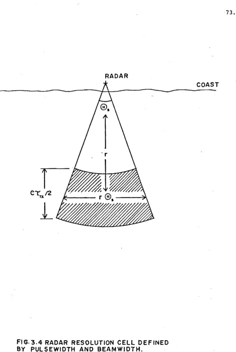
3.4 Radar resolution cell defined by pulsewidth and

beamwidth.

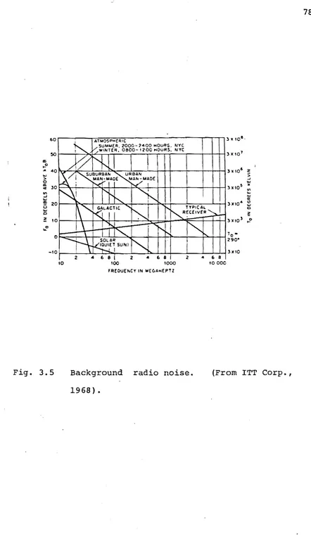
3.5

3.6

Background radio noise.

Analogue and digital spectral analysis techniques.

3.7 Spectrum of 26 MHz sea-echo timeseries rounded to 4 bit accuracy.

4.1

4.2

4.3

Bragg relationship.

Typical form of a sea-echo Doppler spectrum.

Wind direction from Bragg-line ratio.

5.1 Location of the Birdlings Flat field station with

150 antenna beam and radar resolution cell at

5.2

5.3

5.4

30 km.

Layout of Birdlings Flat field station.

PDP-8 computer system and associated hardware.

Coherent frequency generation system.

5.5 Block diagram of coherent 100 kw transmitter

[image:6.595.59.546.64.804.2]

Figure 5.6 6.1 6.2 6.3 6.4 6.5 7.1 7.~ 7.3 8. 1 8.2 8.3

Block diagram of coherent receiving system. Geometry of the propagation problem

Short range ground wave attenuation. a . . . b. Radar performance analysis.

Comparison of measured and predicted echo strengths.

Experimental setup for field strength measurements at Bir6lings Flat.

Overall data collection and processing system. PDP-8 data collection program.

Data collection program timing diagram.

Current broadening of Bragg lines by the variation in the radial component of the current velocity across the radar resolution cell.

Performance of a typical vhf radar system.

a ••• k. A selection of sea-echo Doppler spectra.

CHAPTER 1:

1.1 RADAR REMOTE SENSING OF OCEAN SURFACE CONDITIONS

Over the past decade radar has emerged as a powerful tool for remote sensing of ocean surface conditions. In contrast to traditional techniques which monitor only one point on the

observations}

ocean surface (e. g. buoys and ship radar measurements can obtain data simultaneously from a large number of points over a large area of the ocean surface . . Addit ionally, radar has the potential to measure oceanographic quantities that are difficult or impossible to measure by conventional means. Examples of these quantities are wave direction, variation of current velocity with depth and measurements of wave components travelling in oposition to the wind. The major disadvantages with radar are the large and cumbersome antennas required by some techniques, mutual interference between radar and other users of the electromagnetic spectrum and the fact that radar oceanographic information is not obtained in a direct form as with conventional techniques. Data of interest to oceanographers is only obtained after proper interpretation, and sometimes very complicated analyses of, the radar data. Radar oceanographic techniques can be classified into two groups on the basis of the regions of the electromagnetic spectrum that they use: hf techniques

microwave techniques ~.3-300GHz).

SKYWAVE HF

SATELLITE ALTIMETER (MICROWAVE)

111111111111 (1111111111

GROUND WAVE HF

FI G. 1

.. 1 RADAR OCESl\NOGRAPHY TEC HNI QUES.

SYNTHETIC APERTURE RADAR (MICROWAVE)

4 •

(1 )

hf

techniques.

Conventional

radar

systems

transmit

a

beam

of

elecromagnetic energy which

is

specularly reflected

at perpendicular incidence from the

surface of a

target. This

target is

usually relatively

small.

In contrast

hf

radar

oceanography uses

a

transmitted

beam which

"graz~sll

the

ocean surface at a

very shallow angle.

Energy is, scattered back

to the

reciever by means of an interaction between the radar wave

and the ocean

waves over a relatively large area of the

sea surface.

Radar data are thus averages over

this area

and

extreme events,

such as

the maximum

height of

an

individual wave, cannot

be

measured.

The interaction mechanism responsible

for scattering

the transmitted energy back to the receiver was discovered

in

a pioneering

experiment by

a New

Zealand researcher

(CROMBIE,

1955) •

The

mechanism

is

Bragg scatter,

analogous

to the

Bragg scattering of X-rays

by crystal

structures. Out of

the entire spectrum of

waves present

on

the

ocean

surface

the

radar

energy

reflects most

strongly from those waves with half the wavelength of the

radar.

A simple explanation of this process is that under

these

conditions the

radar

reflections from successive

crests of the ocean wave differ in

phase by

exactly one

wavelength

and

therefore

reinforce.

CROMBIE'S

(1955)

discovery of this Bragg scattering mechanism

provided the

in microwave radar oceanography.

conditions are highly variable, it may not always be possible to obtain a stable propagation path to the point of interest on the sea surface.

With either of these techniques the motion of the Bragg scattering waves on the ocean surface causes the frequency of the received echo to be Doppler shifted from the transmitted frequency. The raw data obtained from hf radar is a Doppler spectrum giving the echo power as a function of Doppler shift from the transmitted carrier. Oceanographic data are obtained by interpreting this Doppler spectrum. Data that have been obtained with hf radar include directional and non-directional ocean waveheight spectra, significant wave height, wind speed and direction, the period and direction of arrival of swell and surface current velocities. The most successful and widely established measurements are the measurement of wind speeds and directions at long ranges using skywave radar (STEWART and BARNUM 1975) and the measurement of surf ace cur rent vectors usi ng groundwave radar (BARRICK eta al., 1977; LIPA and BARRICK, 1983).

7.

rather than the longer gravity waves detected by hf radar. Information on these longer gravity waves is obtained through their modulating effects on the capillary waves. The simplest microwave technique is a conventional radar (i.e. with a rotating beam and plan position indicator display) set up on the coast or on a ship at sea. Radar echoes from ocean waves are often visible as "sea clutter" on the displays of such systems. Under certain conditions images of long period ocean wave trains may be present and from these it is possible to estimate the period and direction of arrival of the waves.

opposed perfectly

to vertical incidence). If the sea smooth

observed back at

a specular reflection will the satellite. Deviations from

surface is not be a 'smooth surface caused by ocean waves, however, will scatter some energy back to the satellite. A scatterometer measures this backscattered energy and determines the ocean waveheight from it.

A satellite or aircraft mounted radar may be used to form an image of the wave pattern on the ocean

means of the synthetic aperture technique. technique the motion of the satellite is

surface by In this used to synthesize a radar antenna much larger than the physical antenna. Due to its size this synthesized antenna has a resolution high enough to detect individual waves. Synthetic aperture radar images can be subject to a two dimensional Four i er tr ansform in order to obtain directional ocean waveheight spectra.

An interesting ground based microwave technique makes use of the Bragg scatter of microwaves from capillary waves mentioned previously. If two closely spaced microwave frequencies are transmitted towards the sea surface an echo is obtained which appears to be due to Bragg scatter of a wave with a frequency equal to the difference between the transmitted frequencies.

effect is due to modulation of-the capillary waves

Bragg scatter the individual frequencies) by longer ocean waves ~hich would Bragg scatter the difference frequency if this frequency had been transmitted directly). By varying the difference between the transmitted frequencies over a suitable range it is thus possible to measure the ocean waveheight spectrum ~LANT, 1977; BARRICK, 1972b).

can obtain data from beyond the line of sight hori zon. The vhf region of the spectrum (30-300MHz) is presently unexplored for the purposes of radar oceanography. We suggest in this work (chapter 8) that a system operating at these frequencies may be able to combine the advantages of compact antennas with microwave systems and over-the-horizon coverage with hf systems.

1.2 AIMS AND SCOPE OF THIS WORK

Two factors influenced the de~cision, to undertake this work. Firstly very little radar oceanography has been done in New Zealand since CROMBIE'S (1955) pioneering work. This is in spite of the fact that there are many potential uses for radar oceanographic information in New Zealand. As examples coastal erosion studies need sea state and wave direction information while Meteorologists are interested in routine monitoring of coastal sea states, In addition weather forcasting in New Zealand is made difficult by the lack of wind speed and direction information from the vast areas of ocean surrounding the country. Skywave hf radars have a proven ability to obtain this information.

tradition of ionospheric and atmospheric research. This

research is carried out at a field station at Birdlings

Flat, a coastal site. As a result echoes from ocean waves

have often been observed ~RASER and VINCENT, 1970).

On the basis of these two factors a trial

investigation of radar oceanography was proposed. The hf

groundwave technique was chosen as:

(a) higher quality spectra are obtained than with the

skywave technique,

~) a wide variety of useful information can be

exracted from these spectra,

(c) The equipment is compatable

existing at Birdlings Flat,

with equipment

~) the antenna systems are simpler and cheaper than

those for skywave systems,

(e) the knowledge gained in the construction of this

system can be directly applied to more elaborate systems

(e.g. skywave or direction finding systems) in the future.

consistent with the requirements of an initial investigation.

The design of a new system at any research establishment always has features and problems unique to that establishment ~urphy's' law!). As a result the emphasis in this work is on the problems inherent in the design, construction and operation of the radar and on the steps leading up to the production of Doppler spectra of sea echo. The radar design information developed during this work is not readily available in the literature and will therefore be of interest to other researchers wishing to develop their own radar systems. In contrast the subsequent analysis of the sea echo Doppler spectra to obtain oceanographic information has been extensively treated in the literature (e.g. BARRICK, 1977 a,b: LIPA and BARRICK, 1980; FORGET et. ala , 1981) and is a relati vely

subj ect to research.

straight-forward data analysis the unique difficulties of

problem not experimental

14.

oceanographers not acquainted with radar theory or, alternatively, radar experts

oceanography. For this reason

not acquainted with a review of the basic principles of oceanography is given in chapter 2 and a review of the theory of pulsed Doppler radars is given in chapter 3. In chapter 3 we also apply the theory of pulsed Doppler radars to the specific case of hf oceanographic·· radars and determine design rules for the basic radar and data analysis parameters. This work, lays the foundations for the groundwave propagation and radar performance analysis work in chapter 6. Chapter 4 combines oceanographic

characteristics

and radar of the sea

theory echo

to outline Doppler spectrum.

CHAPTER

2:

2.1 WAVE MOTION IN THE OCEAN

Wave motion can occur in any physical system in which

a restoring force acts to return some system vari.able to

an equ il ibri urn value. The ocean is no exception to this

rule. A large number of restoring forces gives rise to an

equally large variety of wave motions within the ocean and

on its surf ace. Following MEl (1983) we can classify

these waves according to their restoring force, their

. typical period and the region of the ocean in which they

are found.

The shortest period waves are sound waves. These are

the result of the restoring force provided by the slight

compressibility of sea water and have typical periods

- 2 -5

ran g i ng from 10 to 10 seconds.

Next come capillary waves with periods of the order

of 0.1 seconds. As surface tension provides the restoring

force for these waves they exist only at the interface

between two different media e.g. air and water.

Gravity waves, as their name suggests, arise because

of a restoring force equal to the difference between the

gravitational and bouyant forces on a particle. Due to

~days

.

PI"":'""y

.

: waves

7 6

IP 12

/y

?~/y:

Tides •

·

· .

;

·

_•

·

·

.

long '9fiMIV w...es

·

,

·

I '

.

· .

" •

·

.

: I

·

:

• I

·

: 1

.

• I I

5

TSI.Jf'\3lTlIiS

4 3 log,.(T)

2

10

.

sec

.

&.N'fA

!sec

.

I

Wrd

o

3

-I

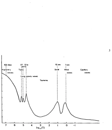
Fig. 2.1. Schematic energy spectrum of oceanic variability. showing the different types of waves occur-ring in the ocean. l.P. denotes the inertial period and is deflIled as n/nlsin¢1. where n magnitude of the Earth's rotation vector and tP is the geographic latitude (Section 3). In this picture I.P. ::= 35 hours,

corresponding to a latitude of i 20·. The relative amplitudes of the various parts of the spectrum do not necessarily reflect actual conditions.

[image:23.595.107.484.53.491.2]

waves are further subdivided on the basis of their generation mechanism. The shortest period gravity waves are generated by the action of wind on the ocean surface and have typical periods ranging from 1 second to 20 seconds. Earthquakes and landslides on the ocean floor generate tsunamis,

ranging from ten

which are gravity waves with periods minutes to over an hour. The final example of surface gravity waves are tides. These are gravity waves with periods of 12 to 24 hours. The driving force for these waves is the gradient of the gravitational attraction of the moon and the sun.

Gravit~ waves are not restricted to the ocean

surface. Variaitons in water density within the ocean (e.g. due to temperature or salinity changes) can provide the bouyant part of the restoring force neccessary for gravity waves to exist. These waves are an important class of waves known as internal waves. Their periods range from a few minutes to half a day_

Coriolis force with latitude actually supplies the restoring force for the wave motion.

Fig. 2.1 (from LeBLOND and MYSAK 1978) is apurely schematic energy spectrum showing the various types of waves that exist on the ocean surface. In this work we will be almost exclusively concerned with wind generated surface gravity waves.

The basic properties of surface gravity waves are given by the first order, linear solution to the equation for irrotational, incompressible fluid motion with gravity and pressure gradient forces acting as the only force terms. Detailed mathematical treatments are given by PHILLIPS (1966), MEl (1983) and LeBLOND and MYSAK (1978). The account given by KINSMAN (1965) is very detailed and gives a great deal of insight into the physical meaning of

the mathematics.

The basic gravity wave solutions are sine waves with wavelength, A , and period, T, related by the dispesion relation:

w2

=

gKtanh(Kd ) 2.1

max where

w ::: _2n/T

and

K

=

2n/A

1000.0

100.0

CD

G)

M ~

G)

a

...

,Q

10.0

....,

QJ)

d

G)

~

G)

~

a

~

1.0

0.1

0.1 1.0 10.0 100.0

Period, seconds

[image:26.595.58.542.103.700.2]

The phase velocity of the wave, v$ by:

51 tanh (Kd )

K max

, is therefore given

. 2.2

Two approximations to the hyperbolic tangent function are possible: When Kd

max tanh ( Kd ) R$ Kd

. max max

is small and when

< 0.33) we have Kd is large we have

max

d max R$

I.

The phase velocity for these two cases becomes:

Kd

max small

2.3 V 2

$

gd max

g/K Kd_max large

Physically, the condition that Kd is small corresponds max

The condi tion that Kd

max is large physicaly corresponds to the condition that the water is deep compared to the wavelength i.e. A < 4 _{d max • The veloci ty}

of these waves is dependant upon their period. i.e. v

=

~ T R:J ( 1 • 5) T ms - 1

<P 2 'IT

and 2.4

Hence deep water waves are dispersive with longer waves travelling faster than shorter waves. A plot of the gravity wave dispersion relation is given in fig. 2.2. The basic properties of deep water waves are illustrated in fig. 2.3. The water particles move in circular orbits. This fact can be easily seen if an object floating in swell is observed. The radius, r, of the circular orbit is equal to the wave amplitude, a, at the surface and decreases exponentially with depth. i.e.

-Kd

r

=

ae 2.5

/

....

FIG 2.3 FIRST ORDER GRAVITY WAVE WITH CIRCULAR ORBITS

OF WATER PARTICLES

A-2rr/tt:.

r-

ae-

Kd

Depth,d

~I

- ;

mean

water

[image:29.842.48.771.54.509.2]

24.

Water waves in shallow water waves move in elliptical orbits with semi-major axis, A, and semi-minor axis, B, given by:

A =

a

d

max +d B

=

a

d max

2.6

Thus the semi-major axis, which is horizontal, stays constant with depth while the vertical semi-minor axis decreases linearly with depth and becomes zero on the ocean floor.

Wave motion usually transports energy from one point to another. In the case of ocean surface waves this energy transport is considerable. MEl (1983) and KINSMAN (1965) show that the energy per unit surface area, E, in a monochromatic surface wave is:

2.1

length of wave crest:

2.8

As a typical example consider a wave with amplitude a

=

1m and period T = lOs •. The surf~ce energy density is 5000

- 2

Jm and the energy flux is 39kW/m. These figures make the current interest in tapping this energy source understandable (SHAW 1982).

2.2 THE OCEAN WAVEHEIGHT SPECTRUM

It is only under very special conditions that the real sea surface approximates the simple sinusoidal form of the first order gravity wave solution. Usualy, in a storm driven sea, the height of the ocean surface above its mean level, n ,is a highly irregular, random function of position and time, n(x, y, t). KINSMAN (1965) gives several excellent photographs showing this random character of the sea surface. In order to represent the sea surface mathematically we consider it to be an interference pattern resulting from the superposition of sinusoidal plane waves of all wavelengths,

A

frequencies, f

=

2n/T, and directions of propagation,

e

Thus we can describe the sea surface as a power spectrum giving the energy in a narrow band of wave components as a function of the wavelengths and frequencies of the components. This spectrum is defined as the Fourier transform of the autocorrelation function of surface waveheight:

S(!5.,W}

=

(2n) 3 1

n (x,y,t) n (x+l1x,y+l1y,

2.9

-iK l1 X -iK l1 Y + iwl1t

t+l1t) > e x y dl1xdl1ydl1t

This spectrum is completely general and can be applied to any time varying rough surface. In particular, the component waves of the spectrum are not restric"ted to first order gravity waves but can be waves resulting from second or higher order hydrodynamic processes. The spectrum is also multi-dimensional, being a function of the two components of spatial wavevector and temporal frequency. Thus numerous forms of ocean waveheight spectra are quoted in the literature (e.g. JOHNSTONE 1975 Ph.D. thesis) corresponding to the many possible ways of reducing the number of dimensions in the spectrum.

If we restrict our attention to first order wave components the dispersion relation (eqn. 2.1) can be used to eliminate one variable from the spectrum to give what is known as the directional ocean waveheight spectrum

i.e. :

S(K ,K ,w) = _S (K

x ' Ky ) 0 (w - IgK) x Y

with _2.10

K

=

IK 2

+

K 2

X _Y

The Cartesian form, S (K , K ) is

x y used mainly in

the normalization condition that both forms, when integrated, must give the same total energy for the ocean surface (JOHNSTONE 1975 Ph.D. thesis). Hence:

S(K ,K )

=

g S (K, S) 2.11

x y ₂

[gK] 3/2

with

K

=

(K ,K )

=

(K, S)

-

x y

tanS

=

K /K

Y x.

We can use the first order dispersion relation' once again to substitute w for K giving the temporal directional ocean waveheight spectr urn S (w,. e) • The s~a surface is now represented by a superposition of many first order waves with frequencies, w _I and propagation directions,

e

The next step in the simplification of these spectra is to integrate out the directional dependa~ce,

e ,

to give non-directional ocean waveheight spectra:

21T

S(K)

=

fS(K/e) dS

0

2.12 21T

S(w) = _{fS(W,S) de}

0

(section 2.5). F~r instance S(w) is the spectrum that would result from spectral analysis of a record of surface height at some point versus time.

Finally, toe. non-directional spectra can· be' integrated to give a single parameter characterising the roughness of the surface. This is the rms waveheight, h:

(Xl

h 2

=

r

S (w) dw

o

2.13

Several other sea state parameters can be related to the rms waveheight. The significant wave height, H

I/3 ' defined as the average height of the largest 1/3 of the waves is given by:

2.14

si gnif i cant wave -height by eqn. 2.14. waveheight is usually denoted Hs.

This significant

The mean waveheight, H , and the average height of the largest 1/10 of the waves are two other commonly used parameters. They are given by ~LACK and HEALY 1981):

-H

=

0.626 HS '

and 2.15

H 1/1 0 = 1. 271 HS

The non-directional ocean waveheight spectrum has uni ts of m2_s

and gives the variance, h2 , of the surface in a narrow band of frequencies. We can convert this variance to energy density by multiplying by the appropriate constants. Hence:

E(w)

=

p 9 S (w) 2.16

_2

is the ocean wave energy spectrum with units Jm sand the total energy density of the ocean surface, in Jm-2 is found by integrating over frequency:

00

E = P g

f

S (w) dw

=

p g h 2 o

Compare this with eqn. 2.8 for the case of a single sinusoidal component.

-2.3 GENERATION OF OCEAN WAVES BY THE WIND

The most common gravity waves on the ocean's surface are generated by the action of wind. The exact mechanism for this p~ocess is, at present, uncertain although some basic details are understod. A simple physical description of the generation of ocean wav~s by the wind may be found in SHEARMAN (1983) while more detailed accounts are given by KINSMAN (1965) and LeBLOND and MYSAK (1978).

An equation for the energy balance of an ocean wave component can be written by considering that the rate of change of surface energy density of the component is due to the nett input of energy from sources and sinks, . W(~) , and the advection of energy away from the area under consideration. Hence:

v .{ (v +v )E(K)}

=

W(K)

c g - 2.18

We have allowed for the possibility that energy may be carried from the region by a current, with velocity Vc ' as well as by natural propagation of energy at the group

of the component. The equilibrium condition will be reached when

aE(K)

=

0

at

for all wave components, K •

The energy sources in the term W(~)

2.19

34.

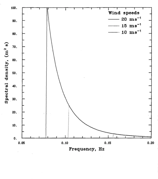
these loss terms. Breaking occurs when the amplitude of the wave becomes so large that the maximum downward acceleration of a particle at the water surface becomes equal to the gravitational acceleration. Any further increase in amplitude will then result in water becoming detached from the surface as foam. The resulting energy loss from breaking thus sets an upper limit to the amplitude of the wave component. PHILLIPS (1958) showed by means of a dimensional argument that this equilibrium, or saturated, amplitude depended only on the wave frequency and not on the wind speed. This equilibrium amplitude is of the form:

S(w) IX w-5 2.20

The wind speed, however, determines a low frequency cutoff point for this relationship as we do not expect much transfer of energy from the wind to wave components travelling faster than the wind to occur.

On the basis of these arguments PHILLIPS (1958 ) proposed the first mathema ti cal expression for the spectrum of a fully developed sea:

f

e :

2

/

W5 _{w ~ glu}

8(w)

=

2.21

Where u is - the wind speed ~/s) and the Phillips saturation constant, Be

,

has been found from comparison with observed spectra to lie in the range

-3 - 2

5xlO - 1.48xlO • A plot of the Phillips spectrum with - 3

Be

=

5xlO and with cutoffs corresponding to different wind speeds is given in fig. 2.4.

Two mechanisms have been proposed for the transfer of energy from the wind to the waves. In the resonant interaction mechanism, energy is fed directly from random fluctuations in air pressure to ocean wave components with the same spatial scale. When the ocean waves become sufficiently developed energy may be transferred by induced interactions in which the waves perturb the flow of air above them to produce pressure variations that are coupled to the wave.

too.

Wind speeds

90.

20

ms-

1

15 ms-

1

80.

. 10 ms-

1

,...

en

_70. ('II

S

..."

..

BO .

.&

...

en

~ 50.

4)

't:J

...

CIS 40.

~ ~

(,)

4)

~ 30.

00

20 •.

to.

O.

0.05 O.tO 0.t5 0.20

Frequency, Hz

[image:42.595.43.563.139.728.2]

37.

longer waves and a concentration of energy in the peak of the spectrum near the cutoff frequency w

=

g/u.

This process has been compared to maser action ~RAUS, 1972).

When compared to observed ocean waveheight spectra the Phillips spectrum, eqn.2.21, is found to have a number of deficiencies. The most important of these is that it applies only to a fully developed sea in which every component has reached its equilibrium amplitude. However considerable time is required for the longer wave components to reach their equilibrium amplitude, and, during this time, these waves will propagate for a large distance because of their high velocities. Therefore the wind must be of sufficient duration and must exist over a sufficient extent of ocean,

for the spectrum to become

known as the fetch, in order fully developed. Spectra for which these conditions are not met are said to be duration limited or fetch limited respectively.

Secondly, observed spectra do not have a cutoff at

w

=

g/u that is as sharp as that implied by the Phillips spectrum. Although very little energy can be transferred directly from the wind to components with greater phase velocities the non-linear processes discussed previously can generate these longer components. As a result the cutoff at w = g/u is much more gradual than that given by

Finally, the Phillips spectrum is a model for the non-directional ocean waveheight spectrum and takes no account of the observed directional properties of ocean wave spectr a.

Many model spectra have been proposed to take account of these difficulties. Most of these spectra were the result of studies in which many observations of actual ocean waveheight spectra were made and a mathematical form developed to provide a good fit to the measured data. BLACK and HEALY (1981) and KINSMAN (1965) provide good accounts of these model spectra and the history of their development. The model spectra can be roughly classified according to which of the three previously mentioned difficulties they attempt to solve.

The problem of non-linear transfer affecting the low frequency cutoff is dealt with by using an exponential function to provide a smoother cutoff. Hence these spectra have the general form:

S (w)

=

A exp

(~)

WS wit

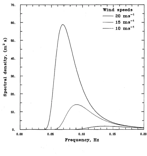
Where A and B are functions of wind speed. At high frequencies they retain the w-5 tail of the Phillips spectrum. A good example of this class of spectra is the Pierson Moskowi t z spectrum (PIERSON and MOSKOWITZ 19.64):

s

(w)

=

exp 2.23

Where we

=

9

lu

is the cu toff f requeney and the constant, v , is empir i cally found to be \!

=

0.74. A plot of this

spectrum for several windspeeds is given in fig. 2.5.

The directional properties of spectra are usualy considered by writing the directional ocean waveheight spectrum as the product of a non-directional spectrum and a directional function, G ( 8) i. e.

S(w,8)

=

S(w) G(8) 2.24

Where 8 = 0 is the wind direction and G ( e) is normalised so that integration of S ( w, 8 oyer angle yields the non-directional spectrum

Se

w) ~qn. 2.12) i.e.

+n

IG(8)d8

=

1 2.25

70.

80.

I"""

50.

CD

('II

S

-...,.I'

..

~ _40.

~

...

CD ~ 4)

'tI

...

30 .

a

J.t ~

()

4)

~

20.

fIJ

iO.

O.

0.00

0.05

O.iO

Frequency, Hz

Wind speeds

20

ms-

1

15

ms-

1

10

ms-

1

O.iS

Fig. 2.5 The Pierson-Moskowitz spectrum.

40.

[image:46.595.53.553.129.661.2]

The simplest direcitonal function is the semi-isotropic form:

1

-TI

G(8)

=

8

TI ~ 8 ~_+ TI

"2

otherwise

Which describes a wave component having

. 2.26

a constant amplitude for all directions within 90 degrees of the wind direction and zero amplitude in directions with a component opposed to the wind direction.

A more gradual decrease of amplitude with direction is provided by an important class of functions with the general form:

G(8)

=

cos s (a8)

N 2.27

Where N is a normalisation constant chosen so that eqn. 2.25 applies. An example is the cardioid distribution which has s

=

2 and a

=

0.5 giving N

=

l/TI • i.e.

G(8)

=

I

This function allows for propagation in all directions except that directly opposing the wind direction, 8

=

n •

Munk (TYLER et .al. 1974) has generalised this torm of the directional dependence to allow the possibility of a different· spread of energy with different frequencies. This is done by wrriting s as a function of frequency:

cos s (8) (e /2)

G(e)

=

N(s)

2.29

The spreading is usualy greater for shorter high frequency waves than for the longer components.

The directional distributions considered so far do not allow any wave propagation directly against the wind

( 8

=

7T). However there is much evidence from radar

studies, including this work, that some energy propagates in the direction 8

=

n even under strong wind conditions (CROMS IE et. al ., 1978; STEWART and TEAGUE, 1980). Munk has allowed for this by further generalising eqn. 2.27 to:

43. Where a typical value for £ is 0.05 (SHEARMAN 1981).Model directional spectra are formed by multiplying these directional distributions with any of the non-directional spectra.

All of the spectra we have been considering so far apply to fully developed seas ~or which the wind has been blowing long enough, and over a sufficient fetch, that each wave component has developed to its equilibrium amplitude. Several models have been proposed that describe the sea under conditions of limited fetch and wind duration. The first of these to come into general use was a wave forecasting system developed by Sverdrup, Munk and Bretschneider ~INSMAN 1965). This system predicted the mean height, H, and mean period of the ocean waves from the wind speed, the wind fetch and the water depth. The duration of the wind was assumed to be infinite.

The most recent fetch limited model spectrum is a result of the Joint North Sea Wave Project (JONSWAP):

2.31

enhancement factor yq and the fact that the parameters specifying this spectrum are functions of fetch. q is given by:

with

w ~w

m w>w

m

2.32

The JONSWAP spectrum is thus specified by the five parameters wm ' ex , y If we define non-dimensional frequency and fetch by:

2.33

-

=

xg/u 2

x 10

(where u is the wind speed measured 10m above the surface) the parameters can be g}ven in terms of the fetch by:

=

3.5 x(-O.33)

ex = 0.076 (2n)

5i

(-0. 22)

y = 0.33 2.34

We have considered the generation of ocean waves by the wind. We now consider what happens to the waves when the wind dies out. As the energy losses from gravity waves are relatively small (below saturation amplitude and particularly at long wavelengths) waves can propagate to very large distances from the storm that generated them. However because gravity waves obey the dispersion relation

~qn. 2.1) longer waves will travel faste~. than ~he.

shorter waves so that the spectrum will become separated out into its component waves. As the spread factor, s, in the directional distribution ~qn. 2.29) decreases with increasing wavelength the long waves at the front of this dispersed wave train will approximate to plane waves. An observer at a distant point in the upwind direction from the storm will see nearly sinusoid waves with long crests and steadily decreasing period. This condition, known as swell, is one of the few instances when the sea surface takes on a regular form.

If the storm occurs at a time t a distance x from o

the observer the time at which waves of frequency w will be observed is given by:

Sincevg

=

g/2w we can rearrange this expression as:

w

=

2.36

47.

2.4 METHODS OF WAVE OBSERVATION

The earliest wave observations came from visual observations from observers on either a ship or the ·coast. These observations were of single parameters such as sea state, average wave period or some measure of wave height

(H, H

,

etc.). The measurement of non-directional ocean

1/3 .

waveheight spectrum, S(

w)

requires a time series of surf ace height relati ve to the mean sea level at a point (i.e.

n

(x,y,t) ). The measurement of S (w) will similarly require a spatial series of height measurements at a fixed point in time. The directional ocean waveheight spectra, S ( K , a) and S ( w , a) will generaly requ ire measurements to be made at many points over an area of the ocean sur face.

suitable for use only in shallow water.

Deep water measurements can be made by using the same transducing systems attached to a vertical, floating spar buoy. This technique uses the fact that wave motion dies out exponentially with depth in deep water. ~qn. 2.5). If the buoy is long and thin then most of its buoyancy will come from those portions of it deep down in the ocean where motion due to the shorter wavelengths is small. It will therefore tend to remain at a constant height with respect to the mean water level. Sometimes a large horizontal disc is attached to the bottom of these buoys to provide additional damping of vertical motion.

If a sinusoidal gravity wave with amplitude, a, is present on the ocean surface pressure fluctuations, with amplitude, 6p, will occur beneath the surface:

6p

=

pga

cosh[K(d+d )] max cosh ~d _{\ max} )

2.37

approximations to eqn. 2.37

-,:d

~ pgae

pga

2.38

We see that in deep water a low pass filtering effect

takes place due to the shorter waves being more rapidly

attenuated with depth than the longer waves. In the

shallow water case the large horizontal water movements

induced by the wave (section 2.2) can cause erroneous measurements due to the ,Bernoulli effect. STEWART (1980)

discusses the conditions under which this e ect will be

important.

An important class of wave measurement techniques

uses measurements of the acceleration of an object

floating in the sea. The height of the surface is obtained,

by integrating the acceleration record twice with respect

to time. Since the mean sea level has zero vertical

acceleration this technique avoids the problem of

providing a reference level and may therefore be used in

deep wa ter. A common example of th is "technique consis ts of

...

a buoy fitted with either a pendulum or a gyroscope in

order to maintain a vertical reference direction. An

accelerometer attached to the pendulum or gyroscope will

acceleration. Rather than integrate this acceleration directly the spectrum of the acceleration, cp (w ), is calculated. From the standard properties of Fourier

transforms it is then easy to show .that the non-directional ocean wavehelght spectrum is given by:

2.39

In another implem entation of the acceleration measurement technique accelerometers are mounted on a ship and measure the response of the ship to the waves. The ocean wave spectrum can then be found from calibrations of

the ship response against an accelerometer buoy.

51.

pendulum. By fitting these measurements to a Taylor series expansion for the water surface the coefficients of the first five terms in a Fourier series expansion for the directional distribution of the ocean waveheight s~ectrum

may be found. If we write the directional spectrum as

S(K,9}

=

G(K,9} S(K} 2.40

Then the buoy data provides coefficients a

i (K), bi(K} such that

G(K,8}

=

2.41

It is interesting to note here that BARRICK and LIPA (1979a) have developed an hf radar technique that obtains these same five coefficients from inversion of the second order component of sea echo Doppler spectra (chapter 3).

52.

array_ Generally the accuracy of this technique

is quite

good provided that only one or two monochromatic waves are

present. Otherwise

the accuracy in the

determination of

the direction of

arrival of

the components falls off

unless the array is made large compared to

the wavelength

of the waves being studied.

In addition

to these wave

observation techniques a

number

of exotic techniques have

been

used

on odd

occasions (STEWART

1980) _

An interes tirig

example

is the

Stereo Wave Observation Project (SWOP)

(KINSMAN

1967).

The

directional ocean waveheight spectrum was measured in this

project by taking stereo pairs of photographs of the ocean

surface from an aircraft. The heights of the surface at a

grid of points covering the

area of the

photograph were

found by using standard techniques of photogrammetry. The

spectrum could then be calculated from a

two dimensional

Fourier transform of this array of heights.

None of these

traditional means for measuring ocean

waveheight spectra is entirely satisfactory. A single

piece of apparatus can obtain measurements from

only one

point or, at most, a limited area

~of

the

ocean surface.

.

.

,

. .

1he equipment is also

d~rectly

exposed to the harsh marine

environment and is liable to damage as a result.

In heavy

seas wave buoys can be pushed directly beneath the surface

with the operation of pole-type recorders and bottom mounted pressure transducers. Expensive underwater cables are sometimes required to connect pressure transducer recorders to the shore. As the size of most devices is much smaller than the wavelength of the waves being measured it is difficult for such devices to have a narrow beam directional response. Directional information is, therefore, limited to uncertainties of the order of ± 45 degrees. Arrays usi~ginterferometric,

beamforming, techniques have much smaller

rather than uncertainties but are limited in the number of directional components they can resolve. Additionally, the interpretation of data from conventional recorders requires care in order to avoid the systematic errors that can occur. KINSMAN

(1967) gives an excellent dscussion of these sources of error.

The hf radar technique has the potential to overcome many of these disadvantages. A single set of equipment can provide simultaneous measurements at a large number of points covering a large area of the 'ocean surface. The equipment is usualy housed in a shore based installation and is therefore protected from damage by the marine environment.

sea state parameters, ocean waveheight spectra, wind speeds and directions, radial components of current velocities and peak frequencies and directions of arrival of swell. The particular parameter measured depends on the way the radar output data is analysed and does not depend much on the configuration of the hardware. Thus records collected to study one particular parameter, e.g. significant wave height, can often be re-analysed at a ter date to extract some other unrelated quantity, e.g. current velocity. with conventional equipment seperate experiments would be needed to measure each of the above q'.Jan ti ties.

Radar can also obtain accurate ( ... ± ID degrees) directional information for both wind driven seas and swell conditions. Under some conditions, however, the directional information may contain ambiguities that would require a second radar or beam direction to resolve. A good example of the use of radar to perform an oceanographic experiment that would otherwise have been difficult or impossible is the work of STEWART and TEAGUE

U98D) on wave growth and decay.

The hf radar technique is not without some disadvantages. Perhaps the most serious of these is that

mutual interference between radar and other users thus appears.

Another problem is that antenna ar rays in the hf band are often large and expensive, particularly if narrow beams are required. This problem provided some of the motivation for the study of the second order part of the sea echo Doppler spectrum and the work by BARRICK and LIPA

(1979a) on compact direction finding antenna systems.

The processing and interpretation of sea echo Doppler spectra can also be difficult. Generally, single parameters are fairly easy to obtain. The extraction of current velocities, wind speeds and wind directions has been particularly successful. Ocean waveheight spectra, however, have to be extracted from the second order part of the Doppler spectrum by using complicated inversion

CHAPTER 3:

PULSED. DOPPLER RADAR

3. 1 DOPP LE R RADARS

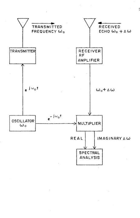
Radar is a technique for measuring properties of a distant object by transmitting electromagnetic energy towards the object and studying the energy that is reflected or scattered by the object. In conventional radar the time delay between transmission and reception of a pulse of energy is used to find the distance, r, to the scattering object. In addition we can get some information on the size and scattering properties of the object from the amplitude of the received echo. The basic principle of Doppler radar is illustrated by the block diagram in fig. 3.1. Here we use the variation in phase of the echo from the object to measure the radial component of the object's velocity. v

=

dr/dt.

If the transmitter transmits a continuous wave with frequency, wo ' and wavenumber, Ko=wo/c, (where c is the speed of light), the complex echo voltage at the receiver input will be of the form:

3.1

We can write this in terms of the phase,~=wot - 2KO~ of the wave as

-iff>

\ / -T-R-A-N-S-M-I''''' .... TTED FREQUENCY We

TR ANSMITIER

\/

...

-RECEIVED

ECHOWe+l:,.W RECEIVER

RF

AMPLIFIER

- jWe

t

e

OSCILLATOR

1---4-I~'

MULTIPLIER

We

-REAL

IMAGINARY l:,.W

FIG 3·, C W DOPPLER RADAR

[image:64.597.58.521.73.791.2]

\/

TRANSM ITTER

...

GATE

""

1\

JL..lf

e

0

OSCILLATOR

Wo

DELAY

l1. t • 2

r

Ie

TRAN SM ITTER TRIGGER

.PULSE

- jw

t

e

0

....

""

\/

RECEIVER R.F

AMPLIFIER

'v

MULTIPLIER

REAL IMAG I NARY

"

\~

RANGE

... _GATES

..

REAL IMAGINARY

:. 'l! \V DOPPLER

~ECTRAL SPECTRUM ANALYSIS I----:;~

FROM RANGE

r

60 • ..

To a first order approximatidn"the received

freqUency,w',

is given by the rate of change of phase with time

dr

dt

3.3

Thus the

received

echo

has "a Doppler shift, w'

=

w

+~~,

o

from the original carrier frequency which

is related to

the radial component of the object's velocity by:

~w

=

- 2K V

o 3.4

This form of the derivation of the Doppler shift equation

stresses the

important point

that

Doppler

veloci ty

information is contained in the phase of the received

signal.

We have considered the case of a single moving target

at range, r.

In Geophysics we are normally interested in

radar scattering from a continuum, such the atmosphere or

ocean, from which reflections are

pro~ced

by many targets

with different ranges and velocities. As a first step in

the treatment of

this problem we

consider the case of

mUltiple targets with different velocities but all at

the

same range from the radar.

Each target will contribute a

of a large number of scatterers; the echo will consist of a continuous spectrum of frequencies,p (w) ,known as the

ex Doppler spectrum.

This Doppler spectrum will consist of a narrow band of frequencies clustered around the transmitted frequency. These Doppler shifts are extreemly small when compared to the transmitted frequency. For the example of hf radar oceanography the Doppler shifts are of the order of 1 Hz with transmitted frequencies of the order of megahertz. The direct measurement of such a spectrum is clearly

impr acti cal. (In addition the AID convertors required to digitise the received signal are limited in frequency response to approximately LMHz.)

We can solve this problem by using the baseband mixing technique (KRENEK 1977 Ph.D. thesis). The received echo voltage~RX(t), is multiplied by the original carrier signal at frequency

v(t)

III o

3.5

By using the shifting property of Fourier transforms (BURDIC 196~ we see that this multiplication shifts the power spectrum of the received echo down in frequency by an amount w

carrier will appear as easily measurable frequencies, 6w

3.6

Physically, this corresponds to forming a beat frequency between the Doppler shifted echo and the carrier frequency.

The echo Doppler spectrum is obtained by performing spectral analysis on the time series of mixer output voltage. The spectral analysis techniques used are the subject of section _3.3. In general the Doppler spectrum will be asymmetrical about OHz and will therefore require the full complex nature of the echo signal to be preserved.

receiver output vol tage at any

convolution of the envelope

time, v _ou t ( t ) , is a

of the transmitted

pulse, v

TX (t) , wi th a function, f (r), describing the

_ scattering properties of the continuum being observed:

vout,t)

=

f

VTX(T)f[~(t-T)J

dT 3.7

-00

In the frequency domain we have:

Pout(W)

=

PTX(w)

I

F(w)

12

3.8

where IF (tl))

12

is the power spectrum of the scattering

function. In order to seperate echoes from ranges spaced

apart by some small amount 6r the receiver output

spectrum must preserve frequency components of the

scattering function within a bandwidth of the order of

c/26r. Thus the condition we must meet in order to

seperate echoes in'range with a resolution 6r is that

the envelope of the transmitted signal must have a

bandwidth of at least:

c

In the time 'domain we can acheive this by short pulse of duration

T TX

given by:

1 26r

= -B

TX c

.

transmitting a

3.10

Transmission of a short pulse is only one of several techniques for generating a wide bandwidth transmittea spectrum. Pulse compression radars ~RENEK, 1979 Ph.D. thesis; BARTON, 1977) achieve very high resolutions with relatively long pulses by using some form of frequency modulation to increase the signal bandwidth.

If we transmit a square pulse of width and assume, without loss of generality, that the surface scattering function has a flat power spectrum then the receiver output spectrum will have a sin ~)/x form with the bandwidth of the main lobe being l/TT'X . In the case of a single transmitted pulse this spectrum will be a continuous spectrum with all frequencies present. Any Doppler shifts of this. spectrum due to target movement will clearly be masked as they are very much smaller than the bandwidth of the spectrum ("'" l~ V s '" 100KH

z )'

of discrete

(f i g 3. 3c) •

lines spaced apart in frequency by f = l/tpr pr

Doppler shifts due to the medium being observed will cause the received echo spectrum to have a copy of a Doppler spectrum at the position of each of these discrete lines. Each Doppler spectrum will be an average over range, the information on the variation in the Doppler spectra with range is contained in the overall envelope. Provided that _{the'spacing of the lines,fpr}

is greater than twice the bandwidth of the Doppler spectra no overlap of the spectra will occur and our aim of

0"

preserving both range and Doppler information will be achieved. The condition that the pulse repetition frequency fpr be greater than twice the Doppler spectrum bandwidth is the Nyquist criterion of signal processing theory (BURDIC 1968).

One practical difficulty remains. In a conventional radar transmitter pulses are formed by turning the carrier frequency oscillator on and off. No attempt is made to control the phase of the oscillator at each pulse. If this phase varies randomly from pulse to pulse the pulse train will not be periodic and its spectrum will be a continuous spectrum such as fig 3.3a. The random variation in phase from pulse -to pulse destroys the

-

..

[image:71.595.61.524.40.771.2]

(0) 5 INGLE RECTANGULAR TRANSMITTED PULSE

WITH LENGTH't'Tx

(b) PHASE COHERENT PULSE TRAIN

(c) MULTIPLIER OUTPUT: RANGE AVERAGED COPIES OF DOPPLER SPECTRA SPACED fpr APART

(d) RANGE GATE OUTPUT~ COPIES OF SPECTRUM FROM ON E RANGE, r

)

j

I

/

"

....

"

V

~

/

'"

/'

V

POWER SPECTRAL DENSITY

-

-....

.... _...

"

,

,

\

fpr='/tpr

o

~

J

V

J

J

\)

o

I

-FIG.3.3 SPECTRA OF PULSED DOPPLER RADAR SIGNALS

' ....

.-67.

repetition frequency are harmonically related (BURDIC 1968). Thus, when the echo spectrum is shifted down to 0 Hz the lowest frequency copy of the Doppler spectrum may be offset from zero by some amount. As a result the subsequent spectral analysis process will have to have a larger bandwidth than would be the case if the Doppler spectrum were centered about zero frequency. We overcome this difficulty by transmitting a phase coherent pulse train in which the pulses are formed by switching, or gating, the signal from a continuously running oscillator into the transmitter power amplifier. There will thus be a linear progression. in carrier phase from one pulse to the next. As BURDIC (1968) shows, the spectrum of a phase coherent pulse train will consist of a series of discrete lines spaced fpr apart and with a line at the carrier frequency, _{f o • The continuously running oscillator from} which this pulse train is derived can also supply the reference signal for the receiver multiplier, thus ensuring that the echo spectrum is shifted down in frequency by exactly the carrier frequency. The effect of the stability of this oscillator on system performance will be discussed further in chapter 5.

68.

circuit and the sample converted into a binarr number

by

an analogue

to digital

(A-Dr' convertor.. The 'sample is

then in a suitable format for processing

by

~

computer.

The range

gate and the A-D track and hold

cir~uit

perform

essentially equivalent functions.

The range

~~te

output

will consist of a series of samples of' the pow<,l' reflected

only from range r.

As illustrated by fig 3.3 the spectrum

of this

sampled

signal

is a

series of cl'pies of the

Doppler spectrum from range r at frequencies sp_1ced

apart

by

f

pr

The

spectrum

is,

in fact, the spr.ctrum of a

sampled version of the continuous signal that would

have

been ob tained

from

a CW Doppler radar if scatterers only

existed at the range r (fig 3.1).

Spectral nnalysis of

this sampled signal thus yields an estimate of the Doppler

spectrum of the echo from just this range.

More than one

range

sample may

be

taken

nfter

each

transmitted pulse,

allowing simultaneous meatlurements of

lhe Doppler spectrum at a number of ranges from the radar.

'1.'he smallest range spacing from which independnll t

Doppler

Apectra may

be

obtained

is

the range resolution of the

radar, !J.r

, whi ch is determined by the tr an6mi

t

ter pulse

length via eqn 3.10.

The echo from range r in an average

bVer this range interval, !J.r

The maximum

r tinge, rmax '

trom

which

echoes

can

be obtained will

be

dotermined by

transmitter power and receiver noise level

con~iderations

In order that echoes from one transmitted pulse do not overlap with subsequent transmitted pulses or their echoes the transmitted pulses must be spaced apart by at least a _{time 2rmax ' c, This condi tion places an upper. limit} on the pulse repetition frequency:

f

= __

c _ pr max 2r max

3.11

We have seen that the Nyquist criterion places a lower limit on fpr of twice the Doppler spectrum bandwidth. In some situations we can have f = f makl" ng

pr min _{pr·max ... ·}

unambiguous determination of range and Doppler shift impossible. Fortunately this conflict does not arise in radar oceanography using ground-wave propagation. Typically, maximum ranges are of the order of 70km and Doppler spectrum bandwidths are no greater than 2Hz (See e.g. BARRICK eta ale 1977). Thus we have

f ~ 2000Hz prmax

3.12

f . R:! 4Hz pr min

We shall show in the following sections that there is considerable advantage in sampling at as high a rate as possible

level of

(J.e. close to f r _{. p maY}} \ in order ba.ckground noise in the spectrum.

70.

3.2 THE RADAR RANGE EQUATION

The power density pr