S.A. Cerri, G. Gouardères, and F. Paraguaçu (Eds.): ITS 2002, LNCS 2363, pp. 388–398, 2002. © Springer-Verlag Berlin Heidelberg 2002
Tutors
Brent Martin and Antonija Mitrovic
Intelligent Computer Tutoring Group
Department of Computer Science, University of Canterbury Private Bag 4800, Christchurch, New Zealand {bim20,tanja}@cosc.canterbury.ac.nz
Abstract. Constraint-Based Modelling (CBM) is a student modelling technique that is rapidly maturing. We have implemented several tutors using CBM and demonstrated its suitability to open-ended domains in particular. A problem with open-ended and complex domain models is their large size, necessitating a comprehensive problem set in order to provide sufficient exercises for extended learning sessions. We have addressed this issue by developing an algorithm that automatically generates new problems directly from the domain knowledge base. We present the algorithm and compare students’ performance with generated problems to those using a teacher-authored problem set, and show the performance of the generated problem set to be superior.
1
Introduction
Constraint-Based Modelling (CBM)
[8]
is an effective approach that simplifies the building of domain and student models. We have used CBM to develop SQL-Tutor[5]
, an ITS for teaching the SQL database language. SQL-Tutor tailors instructional sessions in three ways: by presenting feedback when students submit their answers, by controlling problem difficulty, and by providing scaffolding information. Students have shown significant gains in learning after as little as two hours of exposure to this system[6]
.SQL-Tutor contains a list of questions, from which one is selected that best fits the student’s current knowledge state. In extended sessions with the tutor, the system may run out of suitable problems. We have overcome this by developing a problem generator, which uses the domain model to build new problems that fit the student model. We have implemented this extension to CBM and used it to generate a larger problem set for SQL-Tutor, which has also allowed us to use a problem selection algorithm that is tied more closely to the student model.
2
SQL-Tutor
SQL-Tutor
[5]
teaches the SQL database query language to second and third year students at the University of Canterbury, using Constraint-Based Modelling (CBM). This approach models the domain as a set of state constraints, of the form:If <relevance condition> is true for the student’s solution, THEN <satisfaction condition> must also be true
The relevance condition of each constraint is used to test whether the student’s solution is in a pedagogically significant state. If so, the satisfaction condition is checked. If it succeeds, no action is taken; if it fails, the student has made a mistake and appropriate feedback is given. CBM has advantages over other approaches such as model tracing [1] in that the model need not be complete and correct in order to function. Further, it is well suited to domains where the number of alternative solutions is large or the domain is open-ended.
Ohlsson does not impose any restrictions upon how constraints are encoded, and/or implemented. In SQL-Tutor we initially represented each constraint by a LISP fragment, supported by domain-specific LISP functions. In later versions we have used a pattern-matching algorithm designed for this purpose [4], for example:
(147
"You have used some names in the WHERE clause that are not from this database."
(match SS WHERE (?* (^name ?n) ?*)) (or (test SS (^valid-table (?n ?t))
(test SS (^attribute-p (?n ?a ?t)))) "WHERE")
The syntax of the MATCH function is (MATCH <solution name> <clause> (pattern list)) where <solution name> is either SS (student solution) or IS (ideal solution) and <clause> is the name of the SQL clause to which the pattern applies (e.g. “SELECT”). The pattern list is a set of terms, which match to individual elements in the solution being tested. Each term may be a wildcard, variable, literal or list of literals. The latter denotes that the input element must be a member of the list. Subsequent tests of the value of a variable may be carried out using the TEST function, which is a special form of MATCH that accepts a single pattern term and one or more variables.
Unlike repair theory [9], we make no claim that this algorithm is modelling human behaviour. However, it has the advantage that a failed constraint means that the construct involved is definitely wrong: we do not need to try to infer where the error lies, so our algorithm does not suffer from computational explosion. For further details on this algorithm and the constraint language, see [4].
3
Generating New Problems
In the SQL-Tutor the next problem is chosen based on difficulty, plus the concept the student is currently having the most trouble with. The constraint set is first searched for the constraint that is being violated most often. Then the system identifies the set of problems for which this constraint is relevant. Finally, it choses the problem from this set that best matches the student’s current proficiency level. However, there is no guarantee that an untried problem exists that matches the current student model: there may be no problems for the target constraint, or the only problems available may be of unsuitable difficulty. Further, since the constraint set is large (over 500 constraints), a large number of problems are needed merely to cover the domain. Ideally there should be many problems per constraint, in various combinations. In SQL-Tutor there is an average of three problems per constraint and only around half of the constraint set is covered. A consequence of this is that the number of new constraints (concepts) being presented to the student tapers off as the system runs out of problems. Figure 1 illustrates this. For a six-week open evaluation we found that the number of new constraints presented to the student is linear with the number of problems tackled (R2 = 0.83), until around 40 problems have been solved. At this point the system runs out of suitable problems, and the number of new constraints presented drops to nearly zero.
[image:3.595.133.305.402.580.2]The obvious way to address this limitation is to add more problems. However, this is not an easy task. There are over 500 constraints, and it is difficult to invent problems that are guaranteed to cover all constraints in sufficient combinations that
Fig. 1. New Constraints Applied
0 20 40 60 80 100 120 140 160 180 200
1 7
13 19 25 31 37 43 49 55 61
Problems Solved
Cons
tr
ai
nt
s
A
ppl
ie
there are enough problems at a large spread of difficulty levels. To overcome this we have developed an algorithm that generates new problems from the constraint set. It uses the constraint-based problem solver described in section 2 to create novel SQL statements, using an individual constraint (or, possibly, a set of compatible constraints) as a starting point, and “growing” an SQL statement for which this constraint is relevant. This new SQL statement forms the ideal solution for a new problem. The human author need only convert the ideal solution into a natural language problem statement, ready for presentation to the student.
3.1 Building a New Ideal Solution
To build a new ideal solution we capitalise on the fact that the only reasoning that takes place within a constraint is pattern matching. Each pattern in the relevance condition of a constraint corresponds to a fragment of the solution that must be present for this constraint to be relevant. To create a new ideal solution that is relevant to a particular constraint, we begin by inserting the fragments from this constraint into our (currently blank) ideal solution. Since the pattern matches may contain variables, these must be instantiated. In SQL-Tutor, these variables may correspond to database table or attribute names, literals, relational operators etc. In some cases the value will be constrained by tests in the constraint, which resolve to a set of allowed values. For example, a variable representing a relational operator must contain a member of the set (>, <, <=, >=, =, <> or !=), so the algorithm may immediately instantiate the variable to a random element of this set. In other cases (e.g. literal comparisons, such as “role = ‘Professor Dumbledore’”) there is nothing to limit the value of one or more terms. However, such variables cannot be simply assigned a random value. For example, if the subject of the database being queried is movies, the condition “Title = ‘Star Wars’” would be sensible, but “Title = ‘sekfgdvfv’” would not. To overcome this problem we introduced a small set of further instantiation constraints, which restricts the value of such literals. The instantiation constraints also ensure that semantic consistency is maintained. For example, the instantiation constraint that checks for a valid literal in a comparison is:
(I8
"Ensures that literal string comparisons in WHERE are with valid strings"
(match SS WHERE
(?* (^attribute-of (?n ?a ?t)) "=" (^sql-stringp ?s) ?*))
(test SS (^valid-string (?s ?a ?t)))
"WHERE" )
where “Valid-string” is a macro that enumerates all the valid combinations of attribute names and literal strings. At this stage our new potential ideal solution consists of a set of disjoint fragments, which may or may not be valid SQL.
set problem and syntactic constraints, which simply test that the syntax of the solution is valid. We use this latter set as the input into the constraint-based problem-solver, which corrects any syntactic errors in the ideal solution we have generated so far, leaving a valid SQL query. The result when the problem solver has completed its task is a valid, novel SQL statement, for which the constraint from which it began is relevant. We have thus created a new ideal solution.
3.2 Authoring the New Problem Set
There are two ways we may use the problem generator to develop new exercises: by generating problems on the fly to fit the student model, or by authoring a problem set in advance. While the former gives the greatest flexibility in problem selection (for example, it would allow a problem to be created that fitted the student’s n most problematic constraints), it requires that the system automatically generate the natural language problem text from the ideal solution. This is not an impossible task; however, the problem generation algorithm and the natural language translator would need to be guaranteed robust, otherwise the student may be presented with unintelligible or unsolvable problems. We have therefore adopted the latter approach, and used the algorithm to generate a problem set in advance. This does not preclude the development of a natural language converter; we are designing such a module, again using constraints and the constraint-based problem solver to perform this function.
For the purpose of this study, we used the problem generation algorithm to create a single problem per constraint, giving around 800 potential ideal solutions. We then chose the best of these, and converted them into natural language problem statements. On completion, we had a new problem set of 200 problems, which took only three hours of human effort to build, compared with many days for the human-authored set of 82 problems. Further, when we plotted the number of new constraints applied per problem (the same as the analysis of the control group in Figure 1), the cut-off rose from 40 problems to 60, indicating that the new problem set increased the length of time that a student could fruitfully engage with the system.
4
Evaluation
The motivation for Problem Generation was to reduce the effort involved in building tutoring systems by automating one of the more time-consuming functions; writing the problem set. Three criteria must be met to achieve this goal: the algorithm must work (i.e. it must generate new problems); it must require (substantially) less human involvement than traditional problem authoring; and the problems produced must be shown to facilitate learning to at least the same degree as human-authored problems. The first two were confirmed during the building of the evaluation system: the algorithm successfully generated problems, and the time taken to author the problem set was much less than would have been required for human authoring alone.
learning than the current human-authored set, because we are better able to fit the problem to the student.
SQL-TUTOR was modified for this purpose and evaluated for a six-week period. The subjects were stage two university students studying a databases paper. At the end of the study the students were required to sit a lab test about SQL as part of their assessment, so they were motivated to use the system if they considered it might improve their performance. The students were broken into three groups. The first used the current version of SQL-TUTOR, i.e. with human-authored problems. The second group used a version with problems generated using the algorithm described. The third group used a version containing other research (student model visualisation) that was not relevant to this study. Before using the system, each student sat a pre-test to determine their existing knowledge and skill in writing SQL queries. They were then free to use the system as little or as often as they liked over a six week period. Each student was randomly assigned a “mode”, which determined which version of the system they would use. At the conclusion of the evaluation they sat a post-test.
When the study commenced, 88 students had signed up and performed the pre-test, giving sample sizes of around 30 per group. During the evaluation this further increased as new students requested access to the system. At the conclusion of the study some students who signed up had not used the system to any significant degree. The final groups used for analysis numbered 24 (control) and 26 (experimental) students each. The length of time each student used the system varied greatly from not using it at all to working for several hours, with an average of two-and-a-half hours. Consequently, the number of problems solved also varied widely from zero to 98, with an average of 25.
There are several ways we can measure the performance of the system. First, we can measure the means of the pre-test and post-test, to determine whether or not the systems had differing effects on test performance. Note, however, that with such an open evaluation as this, it is dangerous to assume that differences are due to the system, since use of the system may represent only a portion of the effort the student spent learning SQL. Nevertheless, it is important to analyse the pre-test scores to determine whether the study groups are comparable samples of the population. This was found to be the case.
Second, we can plot the reduction in error rates as the student practices on each constraint. Each student’s performance when measured this way should lead to a so-called ‘Power law’ [2,7], which is typical when the underlying objects being measured (in this case a constraint) represents a concept being learned. The steepness of this curve at the start is a rough indication of the speed with which the student, on average, is learning new constraints. Since each constraint represents a specific concept in the domain, this is an indication of how quickly the student is learning the domain. We can then compare this learning rate between the two groups.
type. If the proportion of problems aborted rises, or the ratio of “too hard” to “too easy” problems is further from 1:1 than the control group, we might conclude that problem difficulty has been adversely affected.
In this study, we measured all of the above. We used the software package SPSS to compare means and estimate power and effect size, and Microsoft Excel to fit power curves. We now present the results.
4.1 Problem Difficulty
We measured problem difficulty both subjectively and objectively. We obtained subjective results by logging when students aborted a problem and recording their reason. If the problems were (overall) of a suitable difficulty, we would expect the ratio of claims of “too hard” to “too easy” to be approximately 1:1. Any significant move away from this ratio would indicate we have adversely affected problem difficulty. Further, the percentage of problems aborted should not rise significantly. Table 1 lists the results. “Aborted” indicates the proportion of all problems attempted that were aborted. “Too hard”, “Too easy” and “Diff type” give the proportion of
aborted problems for which the reason given was the problem was too hard, too easy,
or the student wanted a problem of a different type, respectively. “Responded” indicates the proportion of aborted problems for which the student gave a reason.
These results suggest that for both groups the problems set are more often too easy than too hard. The percentage of problems aborted in each group was exactly the same, at around 26% of all problems. The ratio of “too easy” to “too hard” for the two groups is nearly identical, as is the proportion of problems aborted because the student wanted a problem of a different type. It therefore appears that the generated problems have had no effect on difficulty as perceived by the students.
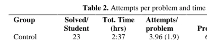
Next, we measured the number of attempts taken to solve each problem. This gives an objective indication of how hard students found the problems. Table 2 lists the results (standard deviations are in parentheses). “Solved/student” indicates the average number of problems completed correctly. “Total time” is the average time spent at the system. This figure records the time that the user was actively using the system, from when they first logged in to when they last submitted an attempt. Thus, it excludes idle time where the user has forgotten to log out. “Attempts per problem” is the number of all submitted attempts (including those for problems the student abandoned), divided by the number of problems actually solved. “Time/Problem” similarly records the total time spent on the system divided by the number of problems solved. There was no significant difference in the objective measurement of problem difficulty: students took approximately the same amount of time and number of attempts in both groups. The number of problems solved and average total time
Table 1. Aborted Problems
Group Aborted
(%)
Too hard (%)
Too easy (%)
Diff Type (%)
Responded (%)
Control 26 24 42 34 84
spent on the system was also almost the same for the two groups, suggesting that neither system was particularly favoured by students.
4.2 Learning Speed
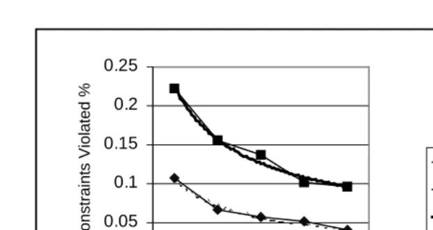
We observed the learning rate for each group by plotting the proportion of constraints that are violated for the nth problem for which this constraint is relevant. This value is obtained by determining for each constraint whether it is correctly or incorrectly applied to the nth problem for which it is relevant. A constraint is correctly applied if it is relevant at any time during solving of this problem, and is always satisfied for the duration of this problem. Constraints that are relevant but are violated one or more times during solving of this problem are labelled erroneous. The value plotted is the proportion of all constraints relevant to the nth problem that are erroneous.
If the unit being measured (constraints in this case) is a valid abstraction of what is being learned, we expect to see a “power curve”. We fitted a power curve to each plot, giving an equation for the curve where the initial learning rate is determined by the slope of the curve at n=1. Note that as the curve progresses learning behaviour becomes swamped by random erroneous behaviour such as slips, so the plot stops trending along the power curve and levels out at the level of random mistakes. This is exacerbated by the fact that the number of constraints being considered reduces as n increases, because many constraints are only relevant to a small number of problems. We therefore use only the initial part of the curve to calculate the learning rate. Figure 2 shows such plots, where each line is the learning curve for the entire group on average, i.e. the proportion of constraints that are relevant to the first problem that are incorrectly applied by any student in the group. The cut-off was chosen at n=5, which is the point at which the power curve fit for both groups is maximal.
[image:8.595.49.387.63.129.2]Both plots exhibit a very good fit to a power curve. The differing slopes of the curves suggest a difference in learning rates between the Problem Generation group and the control group. To determine whether this difference is significant, we plotted curves for each individual student, and used this to determine the initial learning rate of each student. This increases the effect of errors even further, so we determined empirically the best cut-off point for each group, which was found to be n=4. We calculated the learning rate at n=1 for each student, and calculated the mean and significance. Table 3 summarises the results (standard deviations in parentheses).
Table 2. Attempts per problem and time spent
Group Solved/
Student
Tot. Time (hrs)
Attempts/ problem
Time/ Problem (min)
Pre-test mean
Control 23 2:37 3.96 (1.9) 6:14 (3.6) 4.82 (1.5)
Experiment 26 2:31 3.45 (1.2) 5:50 (3.2) 5.06 (1.5)
T-test Significant?
NO (p=0.31)
NO (p=0.71)
Table 3. Initial learning rates
Group Slope Fit (R2)
Control 0.07 (0.04) 0.63 (0.29)
Problem Generation 0.16 (0.12) 0.68 (0.30) T-test significant? YES (p=0.01) NO (p=0.61)
These results show that the slope at n=1, or initial learning rate, is almost twice as high for the experimental group. The difference is statistically significant at a=0.05 (p=0.01). A further test of the results is effect size and power. Using omega squared for effect size [3], we are striving for a power (repeatability) of 0.8, i.e. an 80% likelihood of reproducing this result using the same experimental conditions, and an effect size of around 0.15 (large). Using this method we obtained an effect size of 0.21, with a power of 0.794 at a=0.05, which is a very respectable result.
5
Conclusions
This paper identified the problem of producing enough exercises to tutor students in complex domains. We presented our solution for constraint-based tutors: an algorithm for generating problems directly from the domain model. We described this algorithm, and presented the results of a six-week evaluation using SQL-Tutor, where we aimed to show that the generated problems support learning at least as well as human generated exercises.
The results of the evaluation were extremely encouraging. It appears that the generated problem set improved student’s learning speed by a factor of more than two. The exact cause of this improvement has not been identified; it may be purely because of the increased size of the problem set, or it may be because the problems represented better combinations of constraints. However, either of these is a positive
Probgen: y = 0.2262x-0.5319
R2 = 0.9791 Control:
y = 0.1058x-0.5691 R2 = 0.9697
0 0.05 0.1 0.15 0.2 0.25
1 2 3 4 5
Problems
C
onstraints V
iolated %
Control
Probgen
Pow er (Probgen)
Pow er (Control)
outcome, since increasing the size of the problem set is likely to lead to greater combinations of constraints being represented, and we have shown that it is much easier to author large problem sets using the problem generation algorithm.
The problem generation algorithm does not come without cost. In order for the constraint-based problem solver to work satisfactorily, the constraint set must be sufficiently complete and correct; otherwise the generated solutions (including new ideal ones) may be incorrect. This imposes a greater burden upon the author of the constraint set. However, even this has a positive side: the better the constraint set, the more powerful it will be at diagnosis of student problems. We believe the extra effort is justified, considering the benefits observed.
6
Further Work
We are currently building an authoring system for constraint-based tutors that will incorporate all the various enhancements to CBM that we have developed, including the problem generation algorithm described. We have also begun designing constraints that will convert an SQL ideal solution into the natural language problem statement. If successful, we will incorporate problem statement generation into the authoring tool also.
When authoring the problem set for the study described, we weeded out many problems that were low quality. This arose mainly because of deficiencies in the instantiation constraints. We are looking more closely at this area, to try to identify the required properties of this constraint set, and to determine how it can be more easily deduced.
Acknowledgement. This research was supported by the University of Canterbury
grant U6430.
References
1. Anderson, J. R., Corbett, A. T. and Koedinger, K. R. (1995). Cognitive Tutors: Lessons Learned. Journal of the Learning Sciences 4(2), pp. 167-207.
2. Anderson, J. R. and Lebiere, C. (1998). The atomic components of thought. MahWah, NJ, Lawrence Erlbaum Associates.
3. Chin, D. N. (2001). Empirical Evaluation of User Models and User-Adapted Systems.
User-Modeling and User Adapted Interaction 11, pp. 181-194.
4. Martin, B. and Mitrovic, A. (2000). Tailoring Feedback by Correcting Student Answers. In Gauthier, G., Frasson, C. and VanLehn, K. (Eds.), Proceedings of the Fifth International
Conference on Intelligent Tutoring Systems, Montreal, Springer, pp. 383-392.
5. Mitrovic, A. (1998). Experiences in Implementing Constraint-Based Modeling in SQL-Tutor. In Goettl, B. P., Halff, H. M., Redfield, C. L. and Shute, V. J. (Eds.), Proceedings of
the Fourth International Conference on Intelligent Tutoring Systems, San Antonio, Texas,
Springer, pp. 414-423.
7. Newell, A. and Rosenbloom, P. S. (1981). Mechanisms of skill acquisition and the law of practice. In Cognitive skills and their acquisition. Anderson, J. R. (Ed.), Hillsdale, NJ, Lawrence Erlbaum Associates, pp. 1-56.
8. Ohlsson, S. (1991). Constraint-Based Student Modeling. In Greer, J. and McCalla, G. (Eds.), Proceedings of the NATO Advanced Research Workshop on Student Modelling, Ste. Adele, Quebec, Canada, Springer-Verlag, pp. 167-189.
9. VanLehn, K. (1983). On the Representation of Procedures in Repair Theory. In The
Development of Mathematical Thinking. Ginsburg, H. P. (Ed.), New York, Academic Press,