Average Damage Caused by Multiple Weapons against an Area Target of Normally Distributed Elements

(1)

ISSN Online: 2160-8849 ISSN Print: 2160-8830

DOI: 10.4236/ajor.2017.75022 Sep. 15, 2017 289 American Journal of Operations Research

Average Damage Caused by Multiple Weapons

against an Area Target of Normally

Distributed Elements

Hongyun Wang

1

, George Labaria

1

, Cardy Moten

2

, Hong Zhou

3*

1_{Department of Applied Mathematics and Statistics University of California, Santa Cruz, CA, USA} 2_{TRADOC Analysis Center Naval Postgraduate School, Monterey, CA, USA}

3_{Department of Applied Mathematics Naval Postgraduate School, Monterey, CA, USA}

Abstract

This paper investigates the effect of launching multiple weapons against an area target of normally distributed elements. We provide an analytical form of the average damage fraction and then apply it to obtain optimal aimpoints. To facilitate the computational efforts in practice, we also consider optimizations over given constrained patterns of aimpoints. Finally, we derive scaling laws for optimal aimpoints and optimal damage fraction with respect to the radius of the area target.

Keywords

Area Target, Carleton Damage Function, Average Damage Fraction, Optimal Aimpoints, Scaling Laws

1. Introduction

The theory of firing, which mainly concerns aiming, kill probability and allocation of munitions, was inspired by World War II and has been progressed significantly in the past decades [1]. A brief history of firing theory can be found in Washburn and Kress’s book [2] where the authors also presented a detailed discussion on shooting without feedback or with feedback. Another good reference on weaponeering is given by Driels [3].

In this paper we are interested in studying the effect of precision-guided munitions such as Excaliburs. These coordinate-seeking munitions are usually guided by radio, radar, or laser and launched by a cannon. They are intended to hit a target accurately and cause minimal collateral damage to civilians, friendly

How to cite this paper: Wang, H.Y., Labaria, G., Moten, C. and Zhou, H. (2017) Average Damage Caused by Multiple Weapons against an Area Target of Normally Distri-buted Elements. American Journal of Op-erations Research, 7, 289-306.

https://doi.org/10.4236/ajor.2017.75022 Received: July 4, 2017

Accepted: September 12, 2017 Published: September 15, 2017

(2)

DOI: 10.4236/ajor.2017.75022 290 American Journal of Operations Research

forces and infrastructure, especially hospitals, schools, churches, and residential homes. The precision-guided weapons are in general subject to target-location errors and ballistic dispersion errors. The target-location errors, or aiming errors, result from inaccuracies associated with identifying a target’s location. In contrast, the ballistic dispersion errors are caused by random weapons effects, which may vary from one weapon to another and are assumed to be independent from shot to shot. When a single weapon is fired, it is natural to aim it at the expected center of the target. However, when multiple weapons are launched against a unitary target, the probability of damaging the target can be improved significantly by spreading the aimpoints around the target and the optimal distribution of aimpoints has been investigated in [4] and [5]. Our goal here is to extend our previous studies to estimate the probability of destroying an area target of normally distributed elements with multiple weapons. We will seek optimal aimpoints for various number of weapons.

The plan of this paper is to first review our previous analytical results for the case of multiple weapons against a single target in Section 2. Section 3 introduces the mathematical problem of multiple weapons being released against an area target consisting of normally distributed elements. Exact solution for the average damage fraction is then derived. Section 4 calculates the optimal aiming points and examines the relation among the radius of area target, the number of weapons and the optimal (maximum) damage fraction. In addition to the unconstrained overall optimization of the damage fraction, we also study empirical, fast and robust constrained optimization over several prescribed patterns. The goal is to reduce the computational complexity of optimization and to compute a set of nearly optimal aimpoints efficiently. Section 5 provides scaling laws for optimal aimpoints and optimal damage fraction with respect to the radius of area target. Section 6 highlights conclusions.

2. Review of Our Previous Analytical Results for the Case of

Multiple Weapons against a Single Target

Even though the world is three-dimensional, most targets are known to be on the surface of the Earth and therefore the targets are assumed to be in a two-dimensional ground space. Conventionally, we use two coordinates to define this ground plane: the range direction and the deflection direction. The range direction is defined by the direction of the weapon’s velocity vector, whereas the deflection direction is perpendicular to the range direction.

Previously [5] we have studied the case of multiple weapons with both dependent and independent errors against a single target positioned at xtarget =

( )

0, 0 . For reader’s convenience, we review briefly the mathematical formulation

of the problem. Let

• r_j = the aiming point of weapon j for j=1, 2,,M.

• Y = the dependent error of M weapons, affecting the impact points of all M

(3)

identifying the target location incorrectly/inaccurately. We assume Y is a

normal random variable.

• X_j = independent error of weapon j, affecting only the impact point of

weapon j individually. For example, Xj is the part of error associated with

aiming and firing weapon j. We assume that

{

Xj, j=1, 2,,M

}

are

normal random variables, independent of each other and independent of normal random variable Y .

We model the dependent error Y as a normal random variable with zero

mean: 2 1 2 2 0 0 ~ , 0 0 N

σ

        _{  } _   Y

where σ1 and σ2 are standard deviations, respectively, in the range and the

deflection directions, which give an indication of the spread of the dependent error in these two directions. We model each independent error Xj as a

normal random variable with zero mean:

2 1 2 2 0 0 ~ , 0 0 j d N d         _{  } _   X

The impact point of weapon j is given by

j= + +j j

w r Y X

We use the Carleton damage function described below to model the probability of killing by an individual weapon. Let w=

(

w

( ) ( )

1 ,w 2

)

be the impact point of

a weapon where w

( )

1 and w

( )

2 denote respectively the range component

and the deflection component of the impact point from the target. In Carleton damage function, the probability of the target being killed by a weapon at impact point w is mathematically modeled as

(

)

( )

2

( )

2

2 2

1 2

Pr target being killed by one weapon at impact point

1 2 exp exp 2 2 w w b b ₋  ₋      = _ _ _ _     w (1)

This is the well-known Carleton damage function or the diffuse Gaussian damage function [2]. The two parameters b1 and b2 in the Carleton damage

function (1) represent the effective weapon radii in the range and deflection directions, respectively.

The probability of a target being killed by the M weapons, averaged over all random errors (i.e., dependent and independent errors), is called the kill probability and is mathematically denoted by pkill

(

target,M weapons

)

. Note

that in the notation for the kill probability, the target identity is explicitly included. This will be very convenient later in the discussion of an area target with multiple target elements, in which we can study the kill probability for each individual element.

(4)

{

wj= + +rj Y Xj,j=1, 2,,M

}

, we derived an analytical expression for the kill probability (averaged over the distribution of impact points) as a function of quantities

{

}

(

σ σ1, 2,d d b b1, 2, ,1 2, rj,j=1, 2,,M

)

.

(

)

(

{

}

)

kill target, weapons 1, 2, 1, 2, ,1 2, j, 1, 2, ,

p M =G σ σ d d b b r j=  M (2)

where function G is defined as

{

}

(

)

( )

(1 )

(

)

(

)

1 2 1 2 1 2

1 1 2 1

1 , ,

, , , , , , , 1, 2, ,

1 , , , ,

k j

M k

k k

k j j

G d d b b j M

E F j j E F j j σ σ = =     = −

∑

−

∑

_ _{ } _ r  

  (3)

(

)

(

)

(

)

( )

(

)

( )

(

)

(

)

1

2 2 2

2 ₂

1 1

1

1 1 2 2 2 2 2

1 1 1 1 1

2 2

2

1 1 1

2 2 2 2 2

1 1 1 1 1

, ,

1 1 1

exp

2 2

l l l

k

k k k

j j j

l l l

b d k b

E F j j

b d b d k

r k r k r k

b d k b d k

σ σ = = =  ₊   _{ } _  _{ = } _   ₊ _ ₊ ₊ _  _{ } _ _ _ _ _  − _ _ _ _        × _ − _ + + +      

∑

 (4)

(

)

(

)

(

)

( )

(

)

( )

(

)

(

)

1

2 2 2

2 ₂

2 2

2

2 1 2 2 2 2 2

2 2 2 2 2

2 2

2

1 1 1

2 2 2 2 2

, ,

2 2 2

exp

2 2

l l l

k

k k k

j j j

l l l

b d k b

E F j j

b d b d k

r k r k r k

b d k b d k

σ σ = = =  ₊   _{ } _  _{ = } _   ₊ _ ₊ ₊ _  _{ } _ _ _ _ _  − _ _ _ _        × _ − _ + + +      

∑

 (5)

Mathematically, F1

(

j1,,jk

)

is the product, over k weapons

{

j1,,jk

}

, of

all factors involving only components in the range direction (i.e., σ1, d1, b1,

( )

1

r ) while F₂

(

j₁,,j_k

)

is the product, over k weapons

{

j₁,,j_k

}

, of all

factors involving only components in the deflection direction (i.e., σ2, d2, b2,

( )

2

r ). Together, Equations (2), (3), (4) and (5) form an explicit analytical

expression for the kill probability of a point target, pkill

(

target,M weapons

)

.

This analytical solution will be used in next section to calculate the damage fraction of an area target consisting of normally distributed target elements.

3. Mathematical Formulation: Multiple Weapons against an

Area Target of Normally Distributed Elements

Now let us examine the situation where M weapons are used against an area target centered at xtarget =

( )

0, 0 , consisting of N discrete elements, normally

distributed around the center. Let

• Z_k = the location of element k of the area target, for k=1, 2,,N.

• r_j, X_j, and Y are the same as defined in Section 2. They are respectively,

(5)

DOI: 10.4236/ajor.2017.75022 293 American Journal of Operations Research j.

In this situation, Zk, the location of element k of the area target, is modeled

as a normal random variable with zero mean:

2 1

2 2

0 0 ~ ,

0 0

k

s N

s         _{  } _

 

Z (6)

We assume that

{

Z_k,k=1, 2,,N

}

are independent of each other, and are [image:5.595.259.488.463.679.2]

independent of Xj and Y .

Figure 1 shows a sample distribution for an area target of 20 elements

normally distributed with s1=s2=4.

To study the damage fraction caused by the M weapons on the area target, we examine the kill probability of element k caused by the M weapons. The impact point of weapon j relative to element k of the area target is given by

( )k (k,eff)

j = + +j j− k ≡ +j + j

w r Y X Z r Y X (7)

where the effective dependent error of the M weapons relative to element k is defined as

(k,eff)

k

≡ −

Y Y Z

Note that (k,eff)

Y is a normal random variable with zero mean

( ,eff) 12 12

2 2

0 0

~ , 0 0

k s

N

s

σ

   + 

   

_{  } ₊ _

 

Y

The kill probability of element k caused by the M weapons (averaged over random independent errors

{

Xj, j=1, 2,,M

}

, over the random dependent

error Y , and over the random element location Zk) is given by

(6)

(

)

{

}

(

)

kill

2 2 2 2

1 1 2 2 1 2 1 2

element , weapons

, , , , , , j, 1, 2, ,

p k M

G σ s σ s d d b b j M

= + + r =  (8)

where function G is defined in Equations (3), (4) and (5). Notice that in the case of an area target of normally distributed elements, the kill probability of element

k has exactly the same form as in the case of a single target at

( )

0, 0 with the

exception that all instances of 2 1

σ be replaced by

(

2 2

)

1 s1

σ

+ and 2 2

σ be replaced by

(

2 2

)

2 s2

σ

+ .

Let χk be the Bernoulli random variable indicating whether or not element k is killed (“1” corresponding to “killed”). The damage fraction (random variable) of the area target is the number of elements killed normalized by the total number of elements.

(

)

damage

1 1 area target, weapons

N

k k

q M

N = χ

≡

∑

The average damage fraction has the expression

(

)

(

)

{

}

(

)

damage kill 1 1

2 2 2 2

1 1 2 2 1 2 1 2

area target, weapons

1 1

element , weapons

, , , , , , , 1, 2, ,

N N

k

k k

j

E q M

E p k M

N N

G s s d d b b j M

χ σ σ = =       = _ _=   = + + =

∑

r  (9)

Expression (9) gives the exact solution for the case of an area target of normally distributed elements.

When both the independent error (X_j,j=1, 2,,M ) and the dependent

error (Y ) of the M weapons are absent, random variables

{

χ_k,k=1, 2,,N

}

are independent of each other. In this situation, we can calculate analytically the standard deviation of damage fraction (random variable). The variance of damage fraction has the expression

(

)

[ ]

(

)

damage

2

1 1

var area target, weapons

1 1 1

var var 1

N N

k k

q M

G G

N =χ N = χ N

      = _ _= = − 

∑



∑

(10)

where shorthand notation G is defined as

{

}

(

2 2 2 2

)

1 1, 2 2, 1, 2, ,1 2, j, 1, 2, ,

G≡G σ +s σ +s d d b b r j=  M (11)

The standard deviation of damage fraction is

(

)

(

)

damage

1

std q area target,M weapons G 1 G N

  = −

  (12)

(7)

Note that this expression for the standard deviation is valid only in the absence of dependent and independent errors, for which we have

(

σ σ1, 2,d d1, 2

) (

= 0, 0, 0, 0

)

. When either the independent errors or dependent

error or both are present, the standard deviation of damage fraction is larger than the value predicted by applying Equations (11) and (12) with non-zero

(

σ σ1, 2,d d1, 2

)

. We demonstrate this behavior numerically in Figure 2 and Figure 3. We consider the model problem in which a single shot is fired against an area target of N=20 normally distributed elements. Monte Carlo simulations

are carried out with 106_{runs for each set of parameter values and in each of the}

two situations below (i.e. without or with firing error), yielding accurate numerical results to compare with theoretical predictions.

In Figure 2, there is no firing error; the damage fraction is affected by the radius of area target (the standard deviation of target elements distribution). In this case, both the predicted mean and the predicted standard deviation of damage fraction are valid. As a result, the accurate Monte Carlo simulations agree with the theoretical predictions.

In Figure 3, the radius of area target is fixed at s1=s2 =10; the damage

fraction is affected by the firing error (the total effect of dependent and independent errors; for a single shot, there is no need to distinguish dependent and independent errors). In this case, only the predicted mean of damage fraction is valid. The predicted standard deviation calculated by applying Equations (11) and (12) with non-zero

(

σ σ1, 2,d d1, 2

)

is invalid since Equations (11) and (12) [image:7.595.64.539.437.638.2]

are derived based on the assumption of zero firing error. The right panel of

Figure 2. Statistics of the damage fraction for the case of a single shot against N=20 normally distributed target elements with

(8)

[image:8.595.64.537.57.261.2]

Figure 3. Statistics of the damage fraction for the case of a single shot against N=20 normally distributed target elements with

1 2 10

s =s = , d1=d2=0 and

(

b b1, 2

) (

= 15, 25

)

. The firing error is defined as σ1=σ2. Left panel: mean of damage fraction vs firing error. The analytical expression for the mean is valid regardless of the presence or absence of firing error. Right panel: standard deviation of damage fraction vs firing error. The analytical expression for the standard deviation (Equations (11) and (12)) is valid only in the absence of firing error, which is false for the simulations in this figure. The results of Monte Carlo simulations show that in the presence of firing error, the actual standard deviation of the damage fraction is significantly larger than the value predicted by Equations (11) and (12) (which are not expected to be valid in the presence of firing error).

Figure 3 clearly demonstrates the deviation of the accurate Monte Carlo

simulations from the invalid theoretical prediction.

4. Optimal Aiming Points for an Area Target

Next we investigate the optimal aiming points for the case of multiple weapons against an area target of normally distributed elements. We apply MATLAB built-in function “fminsearch” [6] on Formula (9) to find aiming points which produce the largest damage fraction. Technically MATLAB “fminsearch” yields only a local optimum. To find the global optimum, in each optimization we start MATLAB “fminsearch” with 5 random initial vectors. In all cases of our simulations, all 5 random initial vectors lead to the same optimum, indicating that the optimum found is very likely the global optimum.

(9)

times expensive.

We consider 6 constrained patterns of aiming positions as listed below. These constrained patterns are motivated by the results of overall unconstrained optimization, some of which are shown in Figure 6, Figure 7 and Figure 10.

• _{Pattern A1:}_M_{points on an ellipse, uniform in parameter angle.}

Specifically, the M aiming points are mathematically described by

(

)

1

2π, 1, 2, ,

j

j M

M

θ

= +

θ

− = _ ₍₁₃₎

(

)

1

, cos , sin

j j j j

x y R

η

θ

η

 

= _ _

  (14)

This constrained pattern has three parameters: θ1, R and η, over which

we are going to optimize the average damage fraction. Here θ1 is the parameter

angle for weapon 1. R is the effective radius of the ellipse, satisfying

area of ellipse π

R=

whereas η is the aspect ratio of the ellipse, satisfying

major axis minor axis

η =

• _{Pattern A2: 1 point at center and}

(

M−1

)

points on an ellipse, uniform in

parameter angle.

One aiming point is placed at the center. The rest

(

M−1

)

aiming points are

distributed along an ellipse, uniformly in parameter angle θ, as described by Equations (13) and (14) where M is replaced by

(

M−1

)

. This constrained

pattern has three parameters: θ1, R and η.

• _{Pattern A3: 2 points on the}_x_{-axis and}

(

M−2

)

points on an ellipse,

uniform in parameter angle.

Two aiming points are placed, respectively, at

(

x_a, 0

)

and

(

−x_a, 0

)

. The rest

(

M−2

)

aiming points are distributed along an ellipse, uniformly in parameter

angle θ_{, as described by Equations (13) and (14) where}_M_{is replaced by}

(

M−2

)

. This constrained pattern has 4 parameters: θ₁, R, η, and x_a.

• _{Pattern B1:}_M_{points on an ellipse, uniform in polar angle.}

The M aiming points are mathematically described as follows. Their polar angles φj are given by

(

)

1

2π, 1, 2, ,

j

j M

M

φ

= +

φ

− =  (15)

Their parameter angles θj are determined by the condition that the two

vectors

(

)

1

cos _j, sin _j and cos _j, sin _j point in the same direction

η

θ

φ

η

 

 

  (16)

(10)

(

)

1

, cos , sin

j j j j

x y R

η

θ

η

 

= _ _

  (17)

This constrained pattern contains three parameters: φ1, R and η.

• _{Pattern B2: 1 point at center and}

(

M−1

)

points on an ellipse, uniform in

polar angle.

One aiming point is placed at the center. The rest

(

M−1

)

aiming points are

distributed along an ellipse, uniformly in polar angle φ, as described by Equations (15), (16) and (17) where M is replaced by

(

M−1

)

. This constrained

pattern has three parameters: φ1, R and η.

• _{Pattern B3: 2 points on the}_x_{-axis and}

(

M−2

)

points on an ellipse,

uniform in polar angle.

Two aiming points are placed, respectively, at

(

x_a, 0

)

and

(

−x_a, 0

)

. The rest

(

M−2

)

aiming points are distributed along an ellipse, uniformly in polar angle

φ_{, as described by Equations (15), (16) and (17) where}_M_{is replaced by}

(

M−2

)

. This constrained pattern includes four parameters: φ₁, R, η, and

a

x

.

An example of Pattern B3 (2 points on the x-axis and rest of points on an ellipse, uniform in polar angle) is shown in the left panel of Figure 6. Pattern B1 (all points on an ellipse, uniform in polar angle) and Pattern B2 (1 point at center and rest of points on an ellipse, uniform in polar angle) are illustrated respectively in the left panel and in the right panel of Figure 7.

In numerical simulations below, we choose the parameter values as follows:

1 to 12

M= , number of weapons;

(

b b1, 2

) (

= 60,100

)

, parameters in Carleton damage function;

(

σ σ1, 2

) ( )

= 5, 5 , standard deviation (s.d.) of dependent error in firing errors;

(

d d1, 2

) ( )

= 5, 5 , s.d. of independent errors in firing errors;

1 2 15 to 300

s= =s s = , radius of area target (s.d. of elements distribution).

We compare the results of optimization over constrained patterns with those of the overall optimization. Figure 4 plots the difference in optimal (maximum) damage fraction (popt) between constrained and unconstrained optimizations as

a function of area target radius (s) for various numbers of weapons (M). For small s, the difference in damage fraction is small among various constraints. This is intuitive and reasonable since for small s, the fatal area of each weapon is capable of covering the whole area target. For moderate to large s, the difference in damage fraction compares the performance of optimization constrained over each given pattern. For M ≤6 (Figure 4(a)), the best approximate optimal

damage fraction is achieved by distribute aiming points over an ellipse, uniformly in polar angle (Pattern B1 described above). At M =7 (Figure 4(b)),

the best approximate optimal damage fraction is achieved by placing an aiming point at center and placing the rest six aiming points over an ellipse, uniformly in polar angle (Pattern B2). This is also true for M =8 and M =9. As the

number of weapons increases, at M =10 (Figure 4(c)), the best approximate

(11)

[image:11.595.60.540.65.484.2]

Figure 4. Difference in optimal damage fraction (popt) between constrained and unconstrained optimizations as a function of area target radius (s) for various numbers of weapons (M). (a) M=6; (b) M=7; (c) M=10; (d) M=12.

and the rest eight aiming points over an ellipse, uniformly in polar angle (Pattern B3). The constrained optimum over Pattern B3 remains very accurate at

12

M = weapons (Figure 4(d)).

In summary, as M increases, the best pattern of aiming points for obtaining approximately the highest damage fraction goes from Patterns B1 to B2 to B3. This transition is clearly demonstrated in Figure 5 where the difference in optimal damage fraction (popt) between constrained and unconstrained optimizations is

shown as a function of M at s=150 (radius of area target).

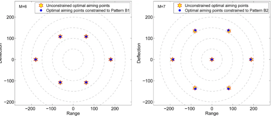
Figure 6 compares the unconstrained optimal aiming points and the optimal

aiming points constrained to Pattern B3, respectively for M =10 and M =12

at s=150. At M =10, the optimal aiming points of Pattern B3 match almost

exactly the unconstrained aiming points. At M =12, the optimal aiming points

(12)

[image:12.595.261.539.58.285.2] [image:12.595.65.538.370.572.2]

Figure 5. Difference in optimal damage fraction (popt) between constrained and unconstrained optimizations as a function of M at s=150 (radius of

area target). In the horizontal direction, all points should have integer values. To visually display points that are on top of each other, they are shifted slightly in the horizontal direction in the plot.

Figure 6. Comparison of unconstrained optimal aiming points and optimal aiming points constrained to Pattern B3. Left panel: two sets of optimal aiming points for M =10, yielding p_{_{opt ,unconstrained}_}=0.772604 and p_{_{opt ,Pattern B3}_}=0.772398, respectively.

Right panel: two sets of optimal aiming points for M =12, yielding p_{_{opt ,unconstrained}_}=0.814997 and p_{_{opt ,Pattern B3}_}=0.813372,

respectively.

discrepancy between these two sets of optimal aiming points, the corresponding damage fractions are still very close to each other: the optimal damage fraction for Pattern B3 is p{opt,Pattern B3}=0.813372 while the overall optimal damage

fraction is p{opt,unconstrained}=0.814997. The difference between these two damage

(13)

computational complexity between these two optimizations. While the constrained optimization over Pattern B3 has 4 variables, the unconstrained optimization for

12

M = weapons has 24 variables, which converges much slower than the

constrained optimization.

The optimal aiming points constrained to Pattern B1 for M =6, the optimal

aiming points constrained to Pattern B2 for M =7 and the corresponding

[image:13.595.67.537.235.436.2]

unconstrained optimal aiming points are displayed in Figure 7.

Figure 8 plots the optimal damage fraction, respectively, as a function of M

for several values of s (left panel), and as a function of s for several values of M

[image:13.595.66.538.497.691.2]

(right panel). For a fixed value of s, the optimal damage fraction increases with

Figure 7. Left panel: unconstrained optimal aiming points and optimal aiming points constrained to Pattern B1 for M=6

weapons. Right panel: unconstrained optimal aiming points and optimal aiming points constrained to Pattern B2 for M=7

weapons.

(14)

the number of weapons, M; for a fixed value of M, the optimal damage fraction decreases as the radius (s) of area target is increased (i.e., damage fraction is lower for a larger area target). Both of these results are reasonable and consistent with our intuition.

[image:14.595.249.500.447.655.2]

A practical question regarding resource allocation is the following: Given the radius of area target (s), what is the minimum number of weapons needed to achieve a given threshold of damage fraction? This question is answered in

Figure 9. Figure 9 shows that for any given threshold of damage fraction, the minimum number of weapons needed is an increasing function of the area target radius (i.e., larger area target requires larger number of weapons), which again is reasonable and consistent with our intuition.

5. Scaling Laws for Optimal Aiming Points and Optimal

Damage Fraction with Respect to Area Target Radius

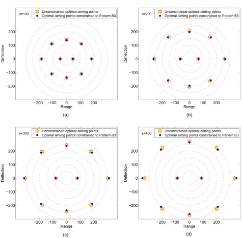
Finally, we study how the optimal aiming points change with s, the radius of area target, and explore if there is a scaling law relating sets of optimal aiming points at different values of s. We start by examining the optimal aiming points for 4 different values of area target radius. The 4 panels in Figure 10 show the optimal aiming points for M = 10 weapons, respectively, for s=100, s=200, s=300

and s=400. The spreading size of optimal aiming points increases as the radius

of area target (s) is increased. However, the increase does not follow a simple proportional linear relationship. Figure 10 indicates that the increase in the spread size of optimal aiming points is less than linear with respect to the area target radius. This can be explained intuitively as follows. When the radius

(15)

[image:15.595.59.537.58.524.2]

Figure 10. Sets of optimal aiming points for M=10 weapons for several values of area target radius (s). (a) s=100; (b) 200

s= ; (c) s=300; (d) s=400.

of area target is increased, the set of aiming points needs to cover a larger region. On the other hand, to maximize the damage fraction, the killing areas associated with individual weapons also need to maintain a certain degree of overlapping with each other. These two needs contradict each other and cannot be both accommodated simultaneously with a fixed number of weapons (M) as the area target radius is increased. Thus, it is expected that as the radius of area target is increased, the spread size of optimal aiming points will increase less than linearly. Here we avoid using the term “radius of optimal aiming points” because the distribution of aiming points is not circularly symmetric.

(16)

we define the size of a set of M aiming points

{

rj, j=1, 2,,M

}

mathematically

as

2 AP

1 1 M

j j L

M =

≡

∑

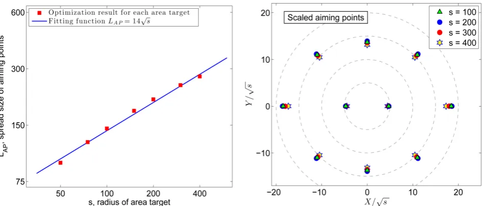
r (18)

To explore how the size of optimal aiming points scales with the area target radius, we plot these two quantities against each other in a log-log plot in the left panel of Figure 11, which also includes a fitting function of the form LAP∝ s.

The log-log plot along the fitting function indicates that the size of optimal aiming points (LAP) approximately is proportional to the square root of area

target radius ( s). These simulation results lead us to the empirical conclusion

that the size of optimal aiming point distribution scales as the square root of area target radius. Based on this key observation, we introduce the scaled aiming points as

(scaled)

( )

1

( )

j s j s

s

≡

r r (19)

The right panel of Figure 11 compares four sets of scaled optimal aiming points of Pattern B3 for s=100, s=200, s=300 and s=400, respectively.

The comparison demonstrates that not only the spread size of optimal aiming points scales as s, the distribution of optimal aiming points after scaling is

approximately invariant with respect to the area target radius. Mathematically, we have observed that approximately

(scaled)

( )

is invariant with respect to

j s s

r (20)

[image:16.595.65.539.475.677.2]

This scaling property gives us an even more efficient way of calculating optimal aiming points. We only need to calculate the optimal aiming points for

Figure 11. Comparison of optimal aiming points for different values of area target radius. Left panel: spread size of optimal aiming points vs. radius of area target in a log-log plot. Right panel: sets of scaled optimal aiming points of Pattern B3 for s=100,

200

(17)

an area target of typical/representative radius:

{

rj

( )

s0 , j=1, 2,,M

}

. We use

0 150

s = in our study. For an area target of radius s, we simply calculate/predict

a set of nearly optimal aiming points from

{

rj

( )

s0

}

using the scaling law.

( )

0

j j

s

s s

s

=

r r (21)

We evaluate the performance of this efficient method by examining the damage fraction values achieved by these sets of nearly optimal aiming points. Specifically, for each area target, we calculate the damage fraction values corresponding respectively to three sets of aiming points:

• _{aiming points calculated in the unconstrained optimization;} • _{aiming points calculated using scaling law (21);}

[image:17.595.64.538.492.675.2]

• _{all aiming points =}

( )

0, 0 .

Figure 12 compares the damage fraction values caused by the 3 sets of aiming points described above for M = 6 weapons (left panel) and for M = 10 weapons (right panel). The damage fraction achieved by the set of nearly optimal aiming points calculated using scaling is indistinguishable from that achieved in the unconstrained optimization (true optimum) while the damage fraction corresponding to all weapons aiming at

( )

0, 0 is much lower. Therefore, we

conclude that scaling law (21) is an efficient and accurate method for calculating a set of nearly optimal aiming points.

6. Concluding Remarks

We have studied the average damage fraction of an area target caused by multiple weapons. The area target was assumed to consist of normally distributed elements. Using the analytical expression of the average damage fraction, we compared various distribution patterns of the aimpoints and gave optimal

Figure 12. Comparison in damage fraction performance of 3 sets of aiming points: 1) aiming points calculated in the unconstrained optimization; 2) aiming points calculated using scaling; and 3) all aiming points =

( )

0, 0 . Left panel: M=6

(18)

patterns for different number of weapons. Scaling laws for optimal aimpoints and optimal damage fraction with respect to the radius of the area target were derived. One prospective future research is to extend our current work to an area target of uniformly distributed elements. Another avenue for future research is to consider an area target where the elements are assigned different values and seek optimal aimpoints in order to minimize the total average surviving value.

Disclaimer

The authors would like to thank TRAC-Monterey for supporting this work and Center for Army Analysis (CAA) for bringing this problem to our attention. The views expressed in this document are those of the authors and do not reflect the official policy or position of the Department of Defense or the U.S. Government.

References

[1] Eckler, A. and Burr, S. (1972) Mathematical Models of Target Coverage and Missile Allocation. Military Operations Research Society,Alexandria, VA.

[2] Washburn, A. and Kress, M. (2009) Combat Modeling. Springer, New York, NY.

https://doi.org/10.1007/978-1-4419-0790-5

[3] Driels, M. (2014) Weaponeering: Conventional Weapon System Effectiveness. 2nd Edition, American Institute of Aeronautics and Astronautics (AIAA) Education Se-ries, Reston, VA.

[4] Washburn, A. (2013) Diffuse Gaussian Multiple-Shot Patterns. Military Operations Research, 8, 59-64

[5] Wang, H., Moten, C., Driels, M., Drundel, D. and Zhou, H. (2016) Explicit Exact Solution of Damage Probability for Multiple Weapons against a Unitary Target.

American Journal of Operations Research, 6, 450-467.

https://doi.org/10.4236/ajor.2016.66042

(19)

Submit or recommend next manuscript to SCIRP and we will provide best service for you:

Accepting pre-submission inquiries through Email, Facebook, LinkedIn, Twitter, etc. A wide selection of journals (inclusive of 9 subjects, more than 200 journals)

Providing 24-hour high-quality service User-friendly online submission system Fair and swift peer-review system

Efficient typesetting and proofreading procedure

Display of the result of downloads and visits, as well as the number of cited articles Maximum dissemination of your research work

Submit your manuscript at: http://papersubmission.scirp.org/

http://www.scirp.org/journal/ajor

: 10.4236/ajor.2017.75022

http://creativecommons.org/licenses/by/4.0/

https://doi.org/10.1007/978-1-4419-0790-5

https://doi.org/10.4236/ajor.2016.66042

https://doi.org/10.1137/S1052623496303470

: http://papersubmission.scirp.org/