Augmenting Neural Networks with First order Logic

292

Augmenting Neural Networks with First-order Logic

Tao Li

University of Utah

[email protected]

Vivek Srikumar

University of Utah

[email protected]

Abstract

Today, the dominant paradigm for training neural networks involves minimizing task loss on a large dataset. Using world knowledge to inform a model, and yet retain the ability to perform end-to-end training remains an open question. In this paper, we present a novel framework for introducing declarative knowl-edge to neural network architectures in order to guide training and prediction. Our frame-work systematically compiles logical state-ments into computation graphs that augment a neural network without extra learnable pa-rameters or manual redesign. We evaluate our modeling strategy on three tasks: ma-chine comprehension, natural language infer-ence, and text chunking. Our experiments show that knowledge-augmented networks can strongly improve over baselines, especially in low-data regimes.

1 Introduction

Neural models demonstrate remarkable predic-tive performance across a broad spectrum of NLP tasks: e.g., natural language inference (Parikh et al.,2016), machine comprehension (Seo et al., 2017), machine translation (Bahdanau et al., 2015), and summarization (Rush et al., 2015). These successes can be attributed to their ability to learn robust representations from data. However, such end-to-end training demands a large num-ber of training examples; for example, training a typical network for machine translation may re-quire millions of sentence pairs (e.g.Luong et al., 2015). The difficulties and expense of curating large amounts of annotated data are well under-stood and, consequently, massive datasets may not be available for new tasks, domains or languages.

In this paper, we argue that we can combat the data hungriness of neural networks by tak-ing advantage of domain knowledge expressed as

Gaius Julius Caesar (July 100 BC – 15 March 44 BC), Roman general, statesman, Consul and notable author of Latin prose, played a critical role in the events that led to the demise of the Roman Republic and the rise of the Roman Empire through his various military campaigns. Paragraph:

Question: Which Roman general is known for writing prose?

Figure 1: An example of reading comprehension that illustrates alignments/attention. In this paper, we con-sider the problem of incorporating external knowledge about such alignments into training neural networks.

first-order logic. As an example, consider the task of reading comprehension, where the goal is to answer a question based on a paragraph of text (Fig. 1). Attention-driven models such as BiDAF (Seo et al.,2017) learn to align words in the question with words in the text as an interme-diate step towards identifying the answer. While alignments (e.g. authortowriting) can be learned from data, we argue that models can reduce their data dependence if they were guided by easily stated rules such as: Prefer aligning phrases that are marked as similar according to an external re-source, e.g., ConceptNet (Liu and Singh,2004). If such declaratively stated rules can be incorporated into training neural networks, then they can pro-vide the inductive bias that can reduce data depen-dence for training.

1. Can we integrate declarative rules with end-to-end neural network training?

2. Can such rules help ease the need for data?

3. How does incorporating domain expertise compare against large training resources powered by pre-trained representations?

The first question poses the key technical chal-lenge we address in this paper. On one hand, we wish to guide training and prediction with neural networks using logic, which is non-differentiable. On the other hand, we seek to retain the advan-tages of gradient-based learning without having to redesign the training scheme. To this end, we propose a framework that allows us to system-atically augment an existingnetwork architecture using constraints about its nodes by deterministi-cally converting rules into differentiable computa-tion graphs. To allow for the possibility of such rules being incorrect, our framework is designed to admit soft constraints from the ground up. Our framework is compatible with off-the-shelf neural networks without extensive redesign or any addi-tional trainable parameters.

To address the second and the third questions, we empirically evaluate our framework on three tasks: machine comprehension, natural language inference, and text chunking. In each case, we use a general off-the-shelf model for the task, and study the impact of simple logical constraints on observed neurons (e.g., attention) for different data sizes. We show that our framework can suc-cessfully improve an existing neural design, es-pecially when the number of training examples is limited.

In summary, our contributions are:

1. We introduce a new framework for incorpo-rating first-order logic rules into neural net-work design in order to guide both training and prediction.

2. We evaluate our approach on three different NLP tasks: machine comprehension, textual entailment, and text chunking. We show that augmented models lead to large performance gains in the low training data regimes.1

1_{The code used for our experiments is archived here:}

https://github.com/utahnlp/layer_augmentation

2 Problem Setup

In this section, we will introduce the notation and assumptions that form the basis of our formalism for constraining neural networks.

Neural networks are directed acyclic compu-tation graphs G = (V, E), consisting of nodes (i.e. neurons) V and weighted directed edgesE that represent information flow. Although not all neurons have explicitly grounded meanings, some nodes indeed can be endowed with semantics tied to the task. Node semantics may be assigned dur-ing model design (e.g. attention), or incidentally discovered in post hoc analysis (e.g., Le et al., 2012;Radford et al.,2017, and others). In either case, our goal is to augment a neural network with

suchnamed neuronsusing declarative rules.

The use of logic to represent domain knowl-edge has a rich history in AI (e.g. Russell and Norvig, 2016). In this work, to capture such knowledge, we will primarily focus on conditional statements of the form L → R, where the ex-pressionLis the antecedent (or the left-hand side) that can be conjunctions or disjunctions of liter-als, and R is the consequent (or the right-hand side) that consists of a single literal. Note that such rules include Horn clauses and their general-izations, which are well studied in the knowledge representation and logic programming communi-ties (e.g.Chandra and Harel,1985).

Integrating rules with neural networks presents three difficulties. First, we need a mapping be-tween the predicates in the rules and nodes in the computation graph. Second, logic is not differen-tiable; we need an encoding of logic that admits training using gradient based methods. Finally, computation graphs are acyclic, but user-defined rules may introduce cyclic dependencies between the nodes. Let us look at these issues in order.

As mentioned before, we will assume named neurons are given. And by associating predi-cates with such nodes that are endowed with sym-bolic meaning, we can introduce domain knowl-edge about a problem in terms of these predicates. In the rest of the paper, we will use lower cased letters (e.g.,ai, bj) to denote nodes in a computa-tion graph, and upper cased letters (e.g., Ai, Bj) for predicates associated with them.

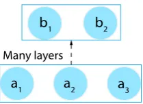
a₁ a₂ a₃ b₁ b₂

Many layers

Figure 2: An example computation graph. The state-mentA1∧B1→A2∧B2is cyclic with respect to the graph. On the other hand, the statementA1∧A2 →

B1∧B2is acyclic.

for compiling conditional statements into differ-entiable statements that augment a given network.

Cyclicity of Constraints Since we will

aug-ment computation graphs with compiled condi-tional forms, we should be careful to avoid creat-ing cycles. To formalize this, let us define cyclicity of conditional statements with respect to a neural network.

Given two nodes a and b in a computation graph, we say that the nodeaisupstreamof node bif there is a directed path fromatobin the graph.

Definition 1 (Cyclic and Acyclic Implications).

Let G be a computation graph. An implicative statementL → R iscyclic with respect to Gif, for any literalRi∈R, the noderiassociated with it is upstream of the nodelj associated with some literalLj ∈L. An implicative statement isacyclic if it is not cyclic.

Fig.2 and its caption gives examples of cyclic and acyclic implications. A cyclic statement sometimes can be converted to an equivalent acyclic statement by constructing its contraposi-tive. For example, the constraint B1 → A1 is

equivalent to¬A1 → ¬B1. While the former is

cyclic, the later is acyclic. Generally, we can as-sume that we have acyclic implications.2

3 A Framework for Augmenting Neural Networks with Constraints

To create constraint-aware neural networks, we will extend the computation graph of an exist-ing network with additional edges defined by con-straints. In §3.1, we will focus on the case where the antecedent is conjunctive/disjunctive and the consequent is a single literal. In §3.2, we will cover more general antecedents.

2_{As we will see in §3.3, the contrapositive does not always}

help because we may end up with a complex right hand side that we can not yet compile into the computation graph.

3.1 Constraints Beget Distance Functions

Given a computation graph, suppose we have a acyclic conditional statement: Z → Y, whereZ is a conjunction or a disjunction of literals andY is a single literal. We define the neuron associated with Y to be y = g(Wx), where g denotes an activation function,Ware network parameters,x

is the immediate input toy. Further, let the vector

zrepresent the neurons associated with the pred-icates inZ. While the nodeszneed to be named neurons, the immediate inputxneed not necessar-ily have symbolic meaning.

Constrained Neural Layers Our goal is to

aug-ment the computation ofy so that wheneverZ is true, the pre-activated value of y increases if the literalY is not negated (and decreases if it is). To do so, we define aconstrained neural layeras

y=g(Wx+ρd(z)). (1)

Here, we will refer to the function d as the dis-tance function that captures, in a differentiable way, whether the antecedent of the implication holds. The importance of the entire constraint is decided by a real-valued hyper-parameterρ≥0.

The definition of the constrained neural layer says that, by compiling an implicative statement into a distance function, we can regulate the pre-activation scores of the downstream neurons based on the states of upstream ones.

Designing the distance function The key

con-sideration in the compilation step is the choice of an appropriate distance function for logical state-ments. The ideal distance function we seek is the indicator for the statementZ:

dideal(z) =

(

1, ifZ holds,

0, otherwise.

However, since the functiondideal is not differen-tiable, we need smooth surrogates.

In the rest of this paper, we will define and use distance functions that are inspired by probabilis-tic soft logic (c.f.Klement et al.,2013) and its use of the Łukasiewicz T-norm and T-conorm to define a soft version of conjunctions and disjunctions.3

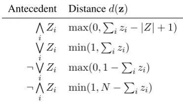
Table 1 summarizes distance functions corre-sponding to conjunctions and disjunctions. In all

3_{The definitions of the distance functions here as}

surro-gates for the non-differentiabledidealis reminiscent of the

Antecedent Distanced(z)

V

i

Zi max(0,Pizi− |Z|+ 1)

W

i

Zi min(1,Pizi)

¬W

i

Zi max(0,1−P

izi) ¬V

i

Zi min(1, N −Pizi)

Table 1: Distance functions designed using the Łukasiewicz T-norm. Here, |Z|is the number of an-tecedent literals. zi’s are upstream neurons associated with literalsZi’s.

cases, recall that thezi’s are the states of neurons and are assumed to be in the range [0,1]. Ex-amining the table, we see that with a conjunctive antecedent (first row), the distance becomes zero if even one of the conjuncts is false. For a dis-junctive antecedent (second row), the distance be-comes zero only when all the disjuncts are false; otherwise, it increases as the disjuncts become more likely to be true.

Negating Predicates Both the antecedent (the

Z’s) and the consequent (Y) could contain negated predicates. We will consider these separately.

For any negated antecedent predicate, we mod-ify the distance function by substituting the corre-spondingzi with1−zi in Table1. The last two rows of the table list out two special cases, where the entire antecedents are negated, and can be de-rived from the first two rows.

To negate consequentY, we need to reduce the pre-activation score of neurony. To achieve this, we can simply negate the entire distance function.

Scaling factorρ In Eq.1, the distance function

serves to promote or inhibit the value of down-stream neuron. The extent is controlled by the scaling factorρ. For instance, withρ = +∞, the pre-activation score of the downstream neuron is dominated by the distance function. In this case, we have a hard constraint. In contrast, with a small ρ, the output state depends on both the Wx and the distance function. In this case, thesoft con-straint serves more as a suggestion. Ultimately, the network parameters might overrule the constraint. We will see an example in §4 where noisy con-straint prefers smallρ.

3.2 General Boolean Antecedents

So far, we exclusively focused on conditional statements with either conjunctive or disjunctive antecedents. In this section, we will consider gen-eral antecedents.

As an illustrative example, suppose we have an antecedent (¬A∨B)∧(C ∨D). By introduc-ing auxiliary variables, we can convert it into the conjunctive formP ∧Q, where(¬A∨B) ↔ P and(C∨D)↔Q. To perform such operation, we need to: (1) introduce auxiliary neurons associated with the auxiliary predicatesPandQ, and, (2) de-fine these neurons to be exclusively determined by the biconditional constraint.

To be consistent in terminology, when consid-ering biconditional statement(¬A∨B)↔P, we will call the auxiliary literalPthe consequent, and the original literalsAandBthe antecedents.

Because the implication is bidirectional in bi-conditional statement, it violates our acyclicity re-quirement in §3.1. However, since the auxiliary neuron state does not depend on any other nodes, we can still create an acyclic sub-graph by defin-ing the new node to be the distance function itself.

Constrained Auxiliary Layers With a

bicondi-tional statementZ ↔ Y, whereY is an auxiliary literal, we define aconstrained auxiliary layeras

y=d(z) (2)

wheredis the distance function for the statement,

zare upstream neurons associated withZ,yis the downstream neuron associated withY. Note that, compared to Eq.1, we do not need activation func-tion since the distance, which is in [0,1], can be interpreted as producing normalized scores.

Note that this construction only applies to aux-iliary predicates in biconditional statements. The advantage of this layer definition is that we can use the same distance functions as before (i.e., Ta-ble 1). Furthermore, the same design consider-ations in §3.1 still apply here, including how to negate the left and right hand sides.

Constructing augmented networks To

Ta-ble1(with appropriate corrections for negations). (3) Use the distance functions to construct con-strained layers and/or auxiliary layers to augment the computation graph by replacing the original layer with constrained one. (4) Finally, use the augmented network for end-to-end training and in-ference. We will see complete examples in §4.

3.3 Discussion

Not only does our design not add any more train-able parameters to the existing network, it also ad-mits efficient implementation with modern neural network libraries.

When posing multiple constraints on the same downstream neuron, there could be combinatorial conflicts. In this case, our framework relies on the base network to handle the consistency issue. In practice, we found that summing the constrained pre-activation scores for a neuron is a good heuris-tic (as we will see in §4.3).

For a conjunctive consequent, we can decom-pose it into multiple individual constraints. That is equivalent to constraining downstream nodes independently. Handling more complex conse-quents is a direction of future research.

4 Experiments

In this section, we will answer the research ques-tions raised in §1by focusing on the effectiveness of our augmentation framework. Specifically, we will explore three types of constraints by augment-ing: 1) intermediate decisions (i.e. attentions); 2) output decisions constrained by intermediate states; 3) output decisions constrained using label dependencies.

To this end, we instantiate our framework on three tasks: machine comprehension, natural lan-guage inference, and text chunking. Across all ex-periments, our goal is to study the modeling flex-ibility of our framework and its ability to improve performance, especially with decreasing amounts of training data.

To study low data regimes, our augmented net-works are trained using varying amounts of train-ing data to see how performances vary from base-lines. For detailed model setup, please refer to the appendices.

4.1 Machine Comprehension

Attention is a widely used intermediate state in several recent neural models. To explore the

augmentation over such neurons, we focus on attention-based machine comprehension models on SQuAD (v1.1) dataset (Rajpurkar et al.,2016). We seek to use word relatedness from external resources (i.e., ConceptNet) to guide alignments, and thus to improve model performance.

Model We base our framework on two

mod-els: BiDAF (Seo et al., 2017) and its ELMo-augmented variant (Peters et al.,2018). Here, we provide an abstraction of the two models which our framework will operate on:

p,q=encoder(p),encoder(q) (3) ←−_a,−→_{a =σ(layers(p,q)) (4)}

y,z=σ(layers(p,q,←−a,−→a)) (5)

where p and q are the paragraph and query re-spectively, σ refers to the softmax activation, ←−a

and−→a are the bidirectional attentions fromq top and vice versa,yandzare the probabilities of an-swer boundaries. All other aspects are abstracted asencoderandlayers.

Augmentation By construction of the attention

neurons, we expect that related words should be aligned. In a knowledge-driven approach, we can use ConceptNet to guide the attention values in the model in Eq.4.

We consider two rules to illustrate the flexibility of our framework. Both statements are in first-order logic that are dynamically grounded to the computation graph for a particular paragraph and query. First, we define the following predicates: Ki,j wordpiis related to wordqjin

Concept-Net via edges {Synonym,DistinctFrom, IsA,Related}.

←−

Ai,j unconstrained model decision that word qj best matches to wordpi.

←−

A0_i,j constrained model decision for the above alignment.

Using these predicates, we will study the impact of the following two rules, defined over a set C of content words in p and q:

R1: ∀i, j∈C, Ki,j → ←−

A0_i,j. R2: ∀i, j∈C, Ki,j∧

←− Ai,j →

←− A0_i,j.

The rule R1 says that two words should be

aligned if they are related. Interestingly, compiling this statement using the distance functions in Ta-ble1is essentially the same as adding word relat-edness as a static feature. The ruleR2is more

%Train BiDAF +R1 +R2 +ELMo +ELMo,R1

10% 57.5 61.5 60.7 71.8 73.0

20% 65.7 67.2 66.6 76.9 77.7

40% 70.6 72.6 71.9 80.3 80.9

100% 75.7 77.4 77.0 83.9 84.1

Table 2: Impact of constraints on BiDAF. Each score represents the average spanF1on our test set (i.e. offi-cial dev set) among3random runs. Constrained mod-els and ELMo modmod-els are built on top of BiDAF. We setρ= 2for bothR1andR2across all percentages.

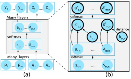
model decision. In both cases, sinceKi,jdoes not map to a node in the network, we have to create a new node ki,j whose value is determined using ConceptNet, as illustrated in Fig.3.

Many

Many layers

layers

a1,1 am,n

.... ....

p₁ p_m q₁ q_n ....

y₁ y_m z1 .... zm

s1,1 sm,n

a1,1 am,n

s1,1 sm,n

s’_1,1 s’m,n

(a) (b)

....

....

....

softmax

a’1,1 .... a’m,n

softmax

softmax

distance

k1,1 km,n

....

Figure 3: (a) The computation graph of BiDAF where attention directions are obmitted. (b) The augmented graph on attention layer using R2. Bold circles are extra neurons introduced. Constrained attentions and scores are a0 and s0 respectively. In the augmented model, graph (b) replaces the shaded part in (a).

Can our framework use rules over named

neu-rons to improve model performance? The

an-swer is yes. We experiment with rules R1 and

R2 on incrementally larger training data.

Perfor-mances are reported in Table 2 with comparison with baselines. We see that our framework can indeed use logic to inform model learning and prediction without any extra trainable parameters needed. The improvement is particularly strong with small training sets. With more data, neural models are less reliant on external information. As a result, the improvement with larger datasets is smaller.

How does it compare to pretrained encoders?

Pretrained encoders (e.g. ELMo and BERT ( De-vlin et al.,2018)) improve neural models with im-proved representations, while our framework

aug-ments the graph using first-order logic. It is im-portant to study the interplay of these two orthog-onal directions. We can see in Table 2, our aug-mented model consistently outperforms baseline even with the presence of ELMo embeddings.

Does the conservative constraintR2help? We

explored two options to incorporate word related-ness; one is a straightforward constraint (i.e. R1),

another is its conservative variant (i.e. R2). It is

a design choice as to which to use. Clearly in Ta-ble 2, constraint R1 consistently outperforms its

conservative alternativeR2, even thoughR2is

bet-ter than baseline. In the next task, we will see an example where a conservative constraint performs better with large training data.

4.2 Natural Language Inference

Unlike in the machine comprehension task, here we explore logic rules that bridge attention neu-rons and output neuneu-rons. We use the SNLI dataset (Bowman et al.,2015), and base our frame-work on a variant of the decomposable atten-tion (DAtt, Parikh et al., 2016) model where we replace its projection encoder with bidirectional LSTM (namely L-DAtt).

Model Again, we abstract the pipeline of

L-DAtt model, only focusing on layers which our framework works on. Given a premisepand a hy-pothesish, we summarize the model as:

p,h=encoder(p),encoder(h) (6) ←−_a,−→_{a =σ(}

layers(p,h)) (7)

y=σ(layers(p,h,←−a,−→a)) (8)

Here, σ is the softmax activation, ←−a and−→a are bidirectional attentions,yare probabilities for la-belsEntailment,Contradiction, andNeutral.

Augmentation We will borrow the predicate

no-tation defined in the machine comprehension task (§4.1), and ground them on premise and hypoth-esis words, e.g. Ki,j now denotes the relatedness between premise wordpiand hypothesis wordhj. In addition, we define the predicateYlto indicate that the label isl. As in §4.1, we define two rules governing attention:

N1: ∀i, j∈C, Ki,j →A0i,j. N2: ∀i, j∈C, Ki,j∧Ai,j →A0i,j.

Intuitively, if a hypothesis content word is not aligned, then the prediction should not be Entail-ment. To use this knowledge, we define the fol-lowing rule:

N3: Z1∨Z2→ ¬YEntail, where

∃j∈C,¬∃i∈C, ←A−0_i,j↔Z1,

∃j∈C,¬∃i∈C, −→A0_i,j

↔Z2.

where Z1 and Z2 are auxiliary predicates tied

to the YEntail predicate. The details of N3 are

illustrated in Fig.4.

a_1,1 a_i,j ....a_m,n

.... ....

p1 pm h1 hn

(a) (b)

s_e s_c s_n y_e y_c y_n

a’1,1 a’i,j ....a’m,n ....

.... softmax

Many

s’e sc sn

z1

y_e y_c y_n

z₂ se softmax

Many layers distance

distance

Many layers layers

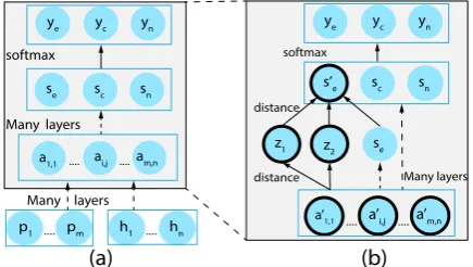
Figure 4: (a) The computation graph of the L-DAtt model (attention directions obmitted). (b) The aug-mented graph on theEntaillabel usingN3. Bold cir-cles are extra neurons introduced. Unconstrained pre-activation scores areswhiles0eis the constrained score

onEntail. Intermediate neurons are z1 andz2.

con-strained attentionsa0 _{are constructed usingN}

1orN2. In our augmented model, the graph (b) replaces the shaded part in (a).

How does our framework perform with large

training data? The SNLI dataset is a large

dataset with over half-million examples. We train our models using incrementally larger percentages of data and report the average performance in Ta-ble3. Similar to §4.1, we observe strong improve-ments from augmented models trained on small percentages (≤10%) of data. The straightforward constraint N1 performs strongly with ≤2% data

while its conservative alternativeN2 works better

with a larger set. However, with full dataset, our augmented models perform only on par with base-line even with lowered scaling factorρ. These ob-servations suggest that if a large dataset is avail-able, it may be better to believe the data, but with smaller datasets, constraints can provide useful in-ductive bias for the models.

Are noisy constraints helpful? It is not always

easy to state a constraint that all examples sat-isfy. ComparingN2 andN3, we see thatN3

per-%Train L-DAtt +N1 +N2 +N3 +N2,3

1% 61.2 64.9 63.9 62.5 64.3 2% 66.5 70.5 69.8 67.9 70.2 5% 73.4 76.2 76.6 74.0 76.4 10% 78.9 80.1 80.4 79.3 80.3 100% 87.1 86.9 87.1 87.0 86.9

Table 3: Impact of constraints on L-DAtt network. Each score represents the average accuracy on SNLI test set among3random runs. For bothN1andN2, we setρ= (8,8,8,8,4)for the five different percentages. For the noisy constraintN3,ρ= (2,2,1,1,1).

formed even worse than baseline, which suggests it contains noise. In fact, we found a significant amount of counter examples toN3during

prelim-inary analysis. Yet, even a noisy rule can improve model performance with ≤10% data. The same observation holds for N1, which suggests

con-servative constraints could be a way to deal with noise. Finally, by comparingN2andN2,3, we find

that the good constraint N2 can not just augment

the network, but also amplify the noise inN3when

they are combined. This results in degrading per-formance in theN2,3 column starting from 5% of

the data, much earlier than usingN3alone.

4.3 Text Chunking

Attention layers are a modeling choice that do not always exist in all networks. To illustrate that our framework is not necessarily grounded to attention, we turn to an application where we use knowledge about the output space to con-strain predictions. We focus on the sequence la-beling task of text chunking using the CoNLL2000 dataset (Tjong Kim Sang and Buchholz, 2000). In such sequence tagging tasks, global inference is widely used, e.g., BiLSTM-CRF (Huang et al., 2015). Our framework, on the other hand, aims to promote local decisions. To explore the interplay of global model and local decision augmentation, we will combine CRF with our framework.

Model Our baseline is a BiLSTM tagger:

x=BiLSTM(x) (9)

y=σ(linear(x)) (10)

wherexis the input sentence,σ is softmax,yare the output probabilities of BIO tags.

Augmentation We define the following

%Train BiLSTM +CRF +C1:5 +CRF,C1:5

5% 87.2 86.6 88.9 88.6 10% 89.1 88.8 90.7 90.6 20% 90.9 90.8 92.1 92.1

40% 92.5 92.5 93.4 93.5

100% 94.1 94.4 94.8 95.0

Table 4: Impact of constraints on BiLSTM tagger. Each score represents the average accuracy on test set of3random runs. The columns of +CRF, +C1:5, and +CRF,C1:5 are on top of the BiLSTM baseline. For

C1:4,ρ= 4for all percentages. ForC5,ρ= 16.

Yt,l The unconstrained decision that tth word has labell.

Y_t,l0 The constrained decision that tth word has labell.

Nt Thetthword is a noun.

Then we can write rules for pairwise label de-pendency. For instance, if wordthas B/I- tag for a certain label, wordt+1can not have an I- tag with a different label.

C1: ∀t, Yt,B-VP → ¬Yt0+1,I-NP

C2: ∀t, Yt,I-NP → ¬Yt0+1,I-VP

C3: ∀t, Yt,I-VP → ¬Yt0+1,I-NP

C4: ∀t, Yt,B-PP → ¬Yt0+1,I-VP

Our second set of rules are also intu-itive: A noun should not have non-NP label.

C5:∀t, Nt→Vl∈{B-VP,I-VP,B-PP,I-PP}¬Yt,l0

While all above rules can be applied as hard constraints in the output space, our framework provides a differentiable way to inform the model during training and prediction.

How does local augmentation compare with

global inference? We report performances in

Table4. While a first-order Markov model (e.g., the BiLSTM-CRF) can learn pairwise constraints such as C1:4, we see that our framework can

better inform the model. Interestingly, the CRF model performed even worse than the baseline with ≤40% data. This suggests that global in-ference relies on more training examples to learn its scoring function. In contrast, our constrained models performed strongly even with small train-ing sets. And by combintrain-ing these two orthogonal methods, our locally augmented CRF performed the best with full data.

5 Related Work and Discussion

Artificial Neural Networks and Logic Our

work is related to neural-symbolic learning (e.g.

Besold et al.,2017) which seeks to integrate neu-ral networks with symbolic knowledge. For exam-ple,Cingillioglu and Russo(2019) proposed neu-ral models that multi-hop logical reasoning.

KBANN (Towell et al.,1990) constructs artifi-cial neural networks using connections expressed in propositional logic. Along these lines, França et al.(2014, CILP++) build neural networks from a rule set for relation extraction. Our distinction is that we use first-order logic toaugmenta given architecture instead of designing a new one. Also, our framework is related toKimmig et al.(2012, PSL) which uses a smooth extension of standard Boolean logic.

Hu et al.(2016) introduced an imitation learn-ing framework where a specialized teacher-student network is used to distill rules into network param-eters. This work could be seen as an instance of knowledge distillation (Hinton et al., 2015). In-stead of such extensive changes to the learning procedure, our framework retains the original net-work design and augments existing interpretable layers.

Regularization with Logic Several recent lines

of research seek to guide training neural networks by integrating logical rules in the form of ad-ditional terms in the loss functions (e.g., Rock-täschel et al.,2015) that essentially promote con-straints among output labels (e.g.,Du et al.,2019; Mehta et al.,2018), promote agreement (Hsu et al., 2018) or reduce inconsistencies across predic-tions (Minervini and Riedel,2018).

Furthermore, Xu et al.(2018) proposed a gen-eral design of loss functions using symbolic knowledge about the outputs. Fischer et al.(2019) described a method for for deriving losses that are friendly to gradient-based learning algorithms. Wang and Poon (2018) proposed a framework for integrating indirect supervision expressed via probabilistic logic into neural networks.

Learning with Structures Traditional

Recently, we have seen some work that allows backpropagating through structures (e.g. Huang et al., 2015; Kim et al., 2017; Yogatama et al., 2017;Niculae et al.,2018;Peng et al.,2018, and the references within). Our framework differs from them in that structured inference is not man-dantory here. We believe that there is room to study the interplay of these two approaches.

6 Conclusions

In this paper, we presented a framework for in-troducing constraints in the form of logical state-ments to neural networks. We demonstrated the process of converting first-order logic into dif-ferentiable components of networks without extra learnable parameters and extensive redesign. Our experiments were designed to explore the flexibil-ity of our framework with different constraints in diverse tasks. As our experiments showed, our framework allows neural models to benefit from external knowledge during learning and predic-tion, especially when training data is limited.

7 Acknowledgements

We thank members of the NLP group at the Uni-versity of Utah for their valuable insights and suggestions; and reviewers for pointers to re-lated works, corrections, and helpful comments. We also acknowledge the support of NSF SaTC-1801446, and gifts from Google and NVIDIA.

References

Martin Anthony. 2003. Boolean functions and artificial neural networks. Boolean Functions.

Dzmitry Bahdanau, Kyunghyun Cho, and Yoshua Ben-gio. 2015. Neural machine translation by jointly learning to align and translate. International Con-ference on Learning Representations.

Tarek R Besold, Artur d’Avila Garcez, Sebastian Bader, Howard Bowman, Pedro Domingos, Pas-cal Hitzler, Kai-Uwe Kühnberger, Luis C Lamb, Daniel Lowd, Priscila Machado Vieira Lima, et al. 2017. Neural-symbolic learning and reason-ing: A survey and interpretation. arXiv preprint arXiv:1711.03902.

Samuel R Bowman, Gabor Angeli, Christopher Potts, and Christopher D Manning. 2015. A large anno-tated corpus for learning natural language inference.

InProceedings of the 2015 Conference on Empirical

Methods in Natural Language Processing.

Ashok K Chandra and David Harel. 1985. Horn clause queries and generalizations. The Journal of Logic Programming, 2.

Ming-Wei Chang, Lev Ratinov, and Dan Roth. 2012. Structured learning with constrained conditional models.Machine learning, 88.

Nuri Cingillioglu and Alessandra Russo. 2019. Deep-logic: End-to-end logical reasoning. AAAI 2019 Spring Symposium on Combining Machine Learning with Knowledge Engineering.

Jacob Devlin, Ming-Wei Chang, Kenton Lee, and Kristina Toutanova. 2018. Bert: Pre-training of deep bidirectional transformers for language under-standing. Proceedings of the 2018 Conference of the North American Chapter of the Association for Computational Linguistics: Human Language Tech-nologies.

Xinya Du, Bhavana Dalvi, Niket Tandon, Antoine Bosselut, Wen tau Yih, Peter Clark, and Claire Cardie. 2019. Be consistent! improving procedural text comprehension using label consistency. In Pro-ceedings of the 2019 Conference of the North Amer-ican Chapter of the Association for Computational Linguistics: Human Language Technologies.

Marc Fischer, Mislav Balunovic, Dana Drachsler-Cohen, Timon Gehr, Ce Zhang, and Martin Vechev. 2019. Dl2: Training and querying neural networks with logic. InInternational Conference on Machine Learning.

Manoel VM França, Gerson Zaverucha, and Artur S d’Avila Garcez. 2014. Fast relational learning us-ing bottom clause propositionalization with artificial neural networks. Machine learning, 94.

Geoffrey Hinton, Oriol Vinyals, and Jeff Dean. 2015. Distilling the knowledge in a neural network. In Neural Information Processing Systems.

Wan-Ting Hsu, Chieh-Kai Lin, Ming-Ying Lee, Kerui Min, Jing Tang, and Min Sun. 2018. A unified model for extractive and abstractive summarization using inconsistency loss. InProceedings of the 56th Annual Meeting of the Association for Computa-tional Linguistics (Volume 1: Long Papers).

Zhiting Hu, Xuezhe Ma, Zhengzhong Liu, Eduard Hovy, and Eric Xing. 2016. Harnessing deep neu-ral networks with logic rules. InProceedings of the 54th Annual Meeting of the Association for Compu-tational Linguistics (Volume 1: Long Papers).

Zhiheng Huang, Wei Xu, and Kai Yu. 2015. Bidirec-tional lstm-crf models for sequence tagging. arXiv preprint arXiv:1508.01991.

Yoon Kim, Carl Denton, Luong Hoang, and Alexan-der M Rush. 2017. Structured attention networks.

InInternational Conference on Learning

Angelika Kimmig, Stephen Bach, Matthias Broecheler, Bert Huang, and Lise Getoor. 2012. A short intro-duction to probabilistic soft logic. InProceedings of the NIPS Workshop on Probabilistic Programming: Foundations and Applications.

Erich Peter Klement, Radko Mesiar, and Endre Pap. 2013. Triangular norms. Springer Science & Busi-ness Media.

Quoc V Le, Marc’Aurelio Ranzato, Rajat Monga, Matthieu Devin, Kai Chen, Greg S Corrado, Jeff Dean, and Andrew Y Ng. 2012. Building high-level features using large scale unsupervised learning. In International Conference on Machine Learning.

Hugo Liu and Push Singh. 2004. ConceptNet – A Prac-tical Commonsense Reasoning Tool-Kit. BT tech-nology journal, 22.

Thang Luong, Hieu Pham, and Christopher D Man-ning. 2015. Effective approaches to attention-based neural machine translation. In Proceedings of the 2015 Conference on Empirical Methods in Natural Language Processing.

Wolfgang Maass, Georg Schnitger, and Eduardo D Sontag. 1994. A comparison of the computational power of sigmoid and boolean threshold circuits. In Theoretical Advances in Neural Computation and Learning, pages 127–151. Springer.

Sanket Vaibhav Mehta, Jay Yoon Lee, and Jaime Car-bonell. 2018. Towards semi-supervised learning for deep semantic role labeling. InProceedings of the 2018 Conference on Empirical Methods in Natural Language Processing.

Pasquale Minervini and Sebastian Riedel. 2018. Ad-versarially regularising neural nli models to inte-grate logical background knowledge. In Proceed-ings of the 22nd Conference on Computational Nat-ural Language Learning.

Vlad Niculae, André FT Martins, Mathieu Blondel, and Claire Cardie. 2018. SparseMAP: Differentiable sparse structured inference. In International Con-ference on Machine Learning.

Xingyuan Pan and Vivek Srikumar. 2016. Expressive-ness of rectifier networks. InInternational Confer-ence on Machine Learning.

Ankur Parikh, Oscar Täckström, Dipanjan Das, and Jakob Uszkoreit. 2016. A decomposable attention model for natural language inference. In Proceed-ings of the 2016 Conference on Empirical Methods in Natural Language Processing.

Adam Paszke, Sam Gross, Soumith Chintala, Gre-gory Chanan, Edward Yang, Zachary DeVito, Zem-ing Lin, Alban Desmaison, Luca Antiga, and Adam Lerer. 2017. Automatic differentiation in pytorch.

InNIPS 2017 Autodiff Workshop.

Hao Peng, Sam Thomson, and Noah A Smith. 2018. Backpropagating through Structured Argmax using a SPIGOT. Proceedings of the 56th Annual Meet-ing of the Association for Computational LMeet-inguistics (Volume 1: Long Papers).

Jeffrey Pennington, Richard Socher, and Christopher Manning. 2014. Glove: Global vectors for word representation. In Proceedings of the 2014 Con-ference on Empirical Methods in Natural Language Processing.

Matthew Peters, Mark Neumann, Mohit Iyyer, Matt Gardner, Christopher Clark, Kenton Lee, and Luke Zettlemoyer. 2018. Deep contextualized word repre-sentations. InProceedings of the 2018 Conference of the North American Chapter of the Association for Computational Linguistics: Human Language Technologies.

Alec Radford, Rafal Jozefowicz, and Ilya Sutskever. 2017. Learning to generate reviews and discovering sentiment.arXiv preprint arXiv:1704.01444.

Pranav Rajpurkar, Jian Zhang, Konstantin Lopyrev, and Percy Liang. 2016. Squad: 100,000+ questions for machine comprehension of text. InProceedings of the 2016 Conference on Empirical Methods in Nat-ural Language Processing.

Matthew Richardson and Pedro Domingos. 2006. Markov logic networks.Machine learning, 62.

Tim Rocktäschel, Sameer Singh, and Sebastian Riedel. 2015. Injecting logical background knowledge into embeddings for relation extraction. InProceedings of the 2015 Conference of the North American Chap-ter of the Association for Computational Linguistics: Human Language Technologies.

Alexander M Rush, Sumit Chopra, and Jason Weston. 2015. A neural attention model for abstractive sen-tence summarization. In Proceedings of the 2015 Conference on Empirical Methods in Natural Lan-guage Processing.

Stuart J Russell and Peter Norvig. 2016. Artificial In-telligence: A Modern Approach. Pearson Education Limited.

Minjoon Seo, Aniruddha Kembhavi, Ali Farhadi, and Hannaneh Hajishirzi. 2017. Bidirectional atten-tion flow for machine comprehension.International Conference on Learning Representations.

Noah A Smith. 2011. Linguistic structure prediction. Synthesis lectures on human language technologies, 4.

Erik F Tjong Kim Sang and Sabine Buchholz. 2000. Introduction to the CoNLL-2000 shared task: Chunking. InProceedings of the 2nd Workshop on Learning Language in Logic and the 4th Conference on Computational Natural Language Learning.

Geoffrey G Towell, Jude W Shavlik, and Michiel O No-ordewier. 1990. Refinement of approximate domain theories by knowledge-based neural networks. In Proceedings of the Eighth National Conference on Artificial Intelligence.

Hai Wang and Hoifung Poon. 2018. Deep probabilis-tic logic: A unifying framework for indirect supervi-sion. InProceedings of the 2018 Conference on Em-pirical Methods in Natural Language Processing.

Jingyi Xu, Zilu Zhang, Tal Friedman, Yitao Liang, and Guy Van den Broeck. 2018. A semantic loss func-tion for deep learning with symbolic knowledge. In International Conference on Machine Learning.

Dani Yogatama, Phil Blunsom, Chris Dyer, Edward Grefenstette, and Wang Ling. 2017. Learning to compose words into sentences with reinforcement learning. InInternational Conference on Machine Learning.

A Appendices

Here, we explain our experiment setup for the three tasks: machine comprehension, natural lan-guage inference, and text chunking. For each task, we describe the model setup, hyperparame-ters, and data splits.

For all three tasks, we used Adam (Paszke et al.,2017) for training and use 300 dimensional GloVe (Pennington et al., 2014) vectors (trained on 840B tokens) as word embeddings.

A.1 Machine Comprehension

The SQuAD (v1.1) dataset consists of 87,599

training instances and10,570development exam-ples. Firstly, for a specific percentage of train-ing data, we sample from the original traintrain-ing set. Then we split the sampled set into 9/1 folds for training and development. The original develop-ment set is reserved for testing only. This is be-cause that the official test set is hidden, and the number of models we need to evaluate is imprac-tical for accessing official test set.

In our implementation of the BiDAF model, we use a learning rate0.001to train the model for20

epochs. Dropout (Srivastava et al., 2014) rate is

0.2. The hidden size of each direction of BiLSTM encoder is100. For ELMo models, we train for

25epochs with learning rate0.0002. The rest hy-perparameters are the same as in (Peters et al.,

2018). Note that we did neither pre-tune nor post-tune ELMo embeddings. The best model on the development split is selected for evaluation. No exponential moving average method is used. The scaling factor ρ’s are manually grid-searched in {1,2,4,8,16} without extensively tuning.

A.2 Natural Language Inference

We use Stanford Natural Language Inference (SNLI) dataset which has549,367training,9,842

development, and9,824test examples. For each of the percentages of training data, we sample the same proportion from the orginal development set for validation. To have reliable model selection, we limit the minimal number of sampled develop-ment examples to be1000. The original test set is only for reporting.

In our implimentation of the BiLSTM variant of the Decomposable Attention (DAtt) model, we adopt learning rate0.0001for100epochs of train-ing. The dropout rate is 0.2. The best model on the development split is selected for evaluation. The scaling factorρ’s are manually grid-searched in {0.5,1,2,4,8,16} without extensively tuning.

A.3 Text Chunking

The CoNLL2000 dataset consists of8,936 exam-ples for training and2,012for testing. From the original training set, both of our training and de-velopment examples are sampled and split (by 9/1 folds). Performances are then reported on the orig-inal full test set.

In our implementation, we set hidden size to