Non-performing loans in European
systemic and non-systemic banks
Ozili, Peterson K
2019
Non-performing loans in European systemic and non-systemic banks
Peterson K. Ozili, PhD.
Abstract
I examine the behaviour of non-performing loans in European systemic and non-systemic banks. The distinction between systemic banks (GSIBs) and non-systemic banks (non GSIBs) is driven by policy reasons. The findings reveal that more profitable banks witness higher non-performing loans regardless of whether they are systemic or non-systemic. Systemic banks have fewer non-performing loans during economic booms and during periods of increased lending while non-systemic banks experience higher NPLs during periods of increased lending. I also observe that European non-systemic banks that exceed regulatory capital requirements have higher NPLs. In the post-2007 financial crisis period, the NPL of systemic banks is negatively associated with the economic cycle which imply that the NPL of systemic banks is procyclical with the state of the economy, and the NPL of systemic banks are positively associated with loan supply and bank profitability. On the other hand, the NPLs of non-systemic banks is negatively associated with regulatory capital ratios, and is positively associated with bank profitability for non-systemic banks in the post-2007 financial crisis period. The findings have implications.
JEL codes: C33, E44, G21
Keywords: credit risk, non-performing loans, systemic banks, systemic risk, impaired loans, asset quality; European banks, Europe, bank profitability.
This Version: 2019
I thank the editors, and two anonymous reviewers for constructive feedback
The views expressed are those of the author and do not necessarily represent the views of the institution(s) the author is affiliated with.
1. Introduction
This study investigates the behaviour of non-performing loans, focusing on the relationship between performing loans (NPLs) and the economic cycle for European systemic and non-systemic banks. The distinction between non-systemic banks (GSIBs) and non-non-systemic (non GSIBs) is driven by policy reasons. In Europe, banking policy makers have growing concern for high non-performing loans in the EU banking sector due to the interdependence between bank financing and economic growth in the European Union (European Commission, 2013, 2014). Also, high levels of NPLs in the European banking sector pose significant risks to financial stability in the EU. The current levels of NPLs piled up in several parts of the EU banking sector are the aftermath of the global financial crisis and sovereign crisis in recent years (European Commission, 2018). Aiyar et al (2015), in an IMF study, show that non-performing loans in the
European Union (EU) stood at about €1 trillion (equivalent to over 9 percent of the GDP of the entire EU region) at the end of 2014 - more than double the level in 2009. They point out that some structural obstacles in the EU banking system discouraged EU banks from addressing their non-performing loan problems, such as prudential supervision issues, legal obstacles, distressed debt markets, informational obstacles, tax and other obstacles.
In addition to these issues, the credit risk of a systemic financial institution in the financial system is crucial for financial system stability. A financial system regulator should be worried if the top ten largest industry obligors or debtors are indebted to systemic banks especially when these loans are non-performing. When high NPLs are concentrated among systemic financial institutions, such losses will be charged against bank profits and can erode bank capital, and the loss of bank capital can lead of the collapse of any financial institution. In recent times, systemic European banks that have serious NPL problems often seek regulatory forbearance from regulators which is a way for them to have more time to deal with their NPL problems.
This study focus on the behaviour of NPLs in European systemic and non-systemic banks because of the systemic risk that distressed too-big-to-fail financial institutions may pose to the entire financial system. The collapse of a systemic bank can collapse the entire financial system, and large performing loans can trigger the failure of a bank. Excess non-performing loans in systemic banks can (i) send the wrong signal to outsiders about the stability of other banks connected to systemic banks (ii) and can bring down any financial institutions if the losses completely wipe out the capital of the bank. Therefore, it is in the best interest of EU policy makers to understand this signalling problem, and they need to address the rising NPL issues in the European banking sector.
This study adopts the Financial Stability Board (FSB) and Basel Committee for Banking Supervision (BCBS)’s distinction between systemic banks (GSIBs) and (non-GSIBs). This classification is used to analyse the behaviour of nonperforming loans in the two bank groups. I analyse European banks over the 2004 to 2013 period, and find that more profitable banks witness higher non-performing loans. Systemic banks have fewer non-performing loans during economic booms and during periods of increased lending while non-systemic banks experience higher NPLs during periods of increased lending. The findings also reveal that systemic banks keep higher regulatory capital ratios when they expect higher NPLs while non-systemic banks that exceed regulatory capital requirements experience higher NPLs.
The study contributes to the literature in the following way. Firstly, this study contributes to the recent literature on the determinants of non-performing loan (Espinoza and Prasad, 2010; Fofack, 2005; Louzis et al, 2012; Ozili, 2019). This study adds to this literature by analysing the link between performing loans and the business cycle, focussing on systemic banks and systemic banks in Europe. An investigation into the behaviour of NPLs in systemic and non-systemic banks is useful for micro-prudential regulation to help EU policy makers understand the implication of large non-performing exposures in systemic and non-systemic banks. Secondly, the analysis in this paper is useful to provide additional insights on the link between problem loans and various states of the economy. Thirdly, this study can help policy makers understand how non-performing loans build-up in systemic financial institutions, and can help policymakers to devise pro-active policy response to quickly address the NPL issues in systemic banks in Europe.
The rest of the paper is organised as follows. Section 2 discuss the literature review on systemic risk measures and the determinants of non-performing loans. Section 3 presents the data. Section 4 discuss the research design and methodology. Section 5 discuss the empirical results. Section 6 concludes.
2. Related Literature
2.1. Measuring Systemic risk
A widely used measure of systemic risk is the conditional value-at-risk (CoVaR) proposed by Adrian and Brunnermeier (2011) which capture risk spill-overs among financial institutions. The CoVar is the value-at-risk (VaR) of the financial system conditional on one institution being in distress (Karimalis and Nomikos, 2018). Another measure of systemic risk is the ‘distressed insurance premium’ (DIP) measure. The distressed insurance premium (DIP) is a hypothetical
insurance premium to cover losses that exceed a certain threshold of banks’ total liabilities
using three approaches: one non-parametric and two different parametric specifications. In comparison, the CATFIN attempts to predict or forecast the macroeconomic systemic risk in the financial sector while the CoVaR and DIP only measure the cross-sectional (bank-level)
differences in banks’ contribution to systemic risk (Allen et al, 2012).
Another systemic risk measure is the component expected shortfall (Banulescu and Dumitrescu, 2015). The component expected shortfall (CES) decompose the risk of the aggregate financial system into several components while accounting for firm characteristics. The CES assess the contribution of a firm to systemic risk at a precise date but also to forecast its contribution over a certain period (Banulescu and Dumitrescu, 2015). The CES is a hybrid measure that combines the ‘Too-Interconnected-To Fail’ and the ‘Too-Big-To-Fail’ logics. Also, CES relies only on publicly available daily data and is similar to the popular ‘Marginal Expected Shortfall’ measure. Another measure of systemic risk is the systemic expected shortfall (SES) by Acharya et al. (2010). The SES is the expected capital shortage of an individual firm conditional on a substantial reduction of the capitalization of the entire system. Under a number of assumptions, SES can be expressed as a linear combination of marginal expected shortfall (MES) and leverage where the parameters of such a combination are not known in general (Brownlees and Engle, 2012). Another measure is the ‘SRISK’ which measures the amount of capital an institution would need to survive a capital shortage in the financial system. It is the amount of capital that a firm would need to survive when the entire system is undercapitalised (Brownlees and Engle, 2012). Similarly, aggregate SRISK is the total amount of capital that the government would need to provide to bailout the financial system in the event of a crisis (Brownlees and Engle, 2012). Other measures include the marginal expected shortfall, etc.
Finally, systemic risk can be measured by whether a financial institution is a global systemically important financial institution or whether it is a non-global systemically important financial institution. The Financial Stability Board (FSB) in 2013 developed a classification for identifying financial institutions that pose the greatest risks to the global financial system. They proposed a G-SIB classification which classify all financial institutions according to their systemic risk contribution to the global financial system. The criteria to determine whether a financial institution is a GSIBs is based on a financial institution (FI)’s size, interconnectedness,
complexity, non-substitutability and cross-border activities (or global reach). This study adopts the G-SIB classification to analyse the behaviour of non-performing loans in banks.
2.2. NPLs and Systemic Risk Regulation – Theoretical Perspectives
For instance, Bleck (2018) argues that when a bank is better informed about its risk than the regulator, any regulation designed to regulate banks would be subject to the Lucas critique. Bleck (2018), building on the Lucas critique, argue that banks know and understand their risk better than regulators, therefore, bank risk-capital regulations are a second-best regulation and might be insensitive to risk. Bleck (2018) supports a leverage ratio-based regulation, and suggest that the leverage ratio of financial institutions might be a better measure for systemic riskiness than risk-based capital regulation.
2.3. Empirical Literature
High NPL ratios can affect bank's short-term and long-term performance through two main channels. First, NPLs generate losses for banks thereby reducing bank profitability and can diminish bank capital when non-performing loans are written-off. In severe cases, high NPLs can make a bank become insolvent. Secondly, high NPLs tie up significant amount of banks' resources, both human and financial, making it difficult for banks to provide new credit to businesses and individuals (European Commission, 2018).
Studies linking credit risk to the state of the economy are not new in the literature (e.g. Carey, 1998; Ruckes, 2004; Salas and Saurina, 2002; Fofack, 2005; Louzis et al, 2012; Ozili and Thankom, 2018). These studies show that in good economic times, banks extend credit to low quality debtors in order to generate higher revenue because the risk of financial distress is usually low during boom years. However, when a recession sets in, non-performing loans are expected to increase for banks. Pesaran (2006) examine the link between changes in credit portfolio and the macroeconomy, and observe that loan default probabilities are strongly driven by the link between firms and the economic cycle, implying that historical data on default probabilities can help predict the likelihood of future non-performing loans. However, data on default probabilities may be difficult to assess for decision making by outsiders. Beck et al (2013) also confirm that data on default probabilities are largely unavailable publicly.
Other studies also use non-performing loan as a measure of bank credit risk. Nkusu (2011), in a panel data analyses, examine the relationship between banks’ loan portfolio quality and macro financial vulnerabilities for 26 countries during 1998 to 2009. Nkusu find a positive relationship between asset quality and the macroeconomic variables used in the study. Glen and Mondragón-Vélez (2011) examine banks from 22 developed countries from 1996 to 2008 and observe that loan loss provisions (a proxy for credit risk) is driven by real GDP growth as well as, low bank capitalisation and private sector leverage. Similarly, Pesola (2005) find a strong link between credit risk and the macroeconomic environment while Drehmann (2005) show that the link between credit risk and macroeconomic shocks may be non-linear. Cihak (2007) and Wezel et al (2014) in their stress-testing analyses examine the resilience of bank balance sheet to adverse economic conditions. These studies suggest that credit risk is strongly linked to changes in the economic cycle.
Quagliarello (2007) observe that the state of the economy is a determinant of non-performing loans for Italian banks. Klein (2013) also document a strong negative relationship between non-performing loans and the economic cycle proxy by change in gross domestic product for banks in Central, Eastern and South- Eastern Europe (CESEE) countries. Fofack (2005) find similar evidence for banks in sub-Saharan African countries while Louzis et al (2012) find similar evidence in the Greek banking sector. Prior literature has not focussed on the link between non-performing loans and the economic cycle for systemic banks compared to non-systemic banks. This present study, in contrast, examine two categories of European banks: systemic banks and non-systemic banks.
3. Data
Pooled cross-section and time series balance sheet data for European banks were collected from the Van Dijk Bankscope database for 16 counties in Europe: United Kingdom, Germany, Ireland, Luxemburg, Norway, Denmark, Finland, Greece, Portugal, Belgium, Netherland, Sweden, Spain, France, Italy and Austria. The sample period covers 2004 to 2013. The rationale for the choice of sample period is to allows us cross-check how the 2007-2008 financial crisis affected systemic and non-systemic banks and also how they have changed since the crisis. Also, since the 2004 to 2013 period precede the date the European Central Bank (ECB) assumed responsibility for the Euro Area banking sector in November 4, 2014, the current sample period will allow us to capture the behaviour of NPLs before the European Central Bank (ECB) intervention.
To control for the 2008 financial crisis, 2008 bank-year observations were eliminated so that the impact of the financial crisis would not affect the validity of the inference(s). A binary dummy variable is introduced to distinguish between the pre-crisis and the post-crisis period. Data for real gross domestic product growth rate, a proxy for economic cycle, is obtained from the World Economic Forum database. The ∆GDP data allows us to detect whether the magnitude of non-performing loans and its link to the economic cycle during the period warranted the full intervention of the European Central Bank in the first place.
The European banks are then divided into systemic (G-SIBs) and non-systemic banks (non-G-SIBs). The distinction between systemic and non-systemic banks is based on the joint Financial
4. Methodology
The multivariate model employed to investigate the relationship between non-performing loans and the economic cycle is a variation of the model used by Beck et al (2013) and Ozili (2019) who examine the determinants of non-performing loans. The functional form of the model in this study is given as
𝑁𝑃𝐿𝑖𝑡 = 𝛽0 + 𝛽1𝐿𝑂𝐴𝑁𝑖𝑡 + 𝛽2𝐶𝐴𝑅𝑖𝑡 + 𝛽3𝐸𝐵𝑇𝑃𝑖𝑡 + 𝛽𝐺𝐷𝑃𝑖, 𝑡 − 1 + 𝛽5𝐺𝐷𝑃𝑖𝑡 + 𝑃𝐸𝑅𝐼𝑂𝐷𝑑𝑢𝑚𝑚𝑖𝑒𝑠 + 𝑒𝑖𝑡.
Where
NPL = Non-performing loan to gross loan ratio for bank i at time t.
LOAN = Change in gross loan outstanding for bank i at time t
CAR = ratio of Tier 1 capital divided by risk-weighted assets for bank i at time t.
EBTP = ratio of earnings before tax and loan loss allowance divided by total assets for bank i at time t.
∆GDP = Real gross domestic product growth rate.
The non-performing loans to gross loans ratio is the dependent variable and the measure of asset quality in the study. The explanatory variables are LOAN, CAR, EBTP and ∆GDP. The LOAN variable is introduced to control for the influence of bank lending on non-performing loans. A negative sign for the LOAN coefficient is expected. The second explanatory variable is regulatory capital ratio. Banks that keep higher regulatory capital ratios will restrain from engaging in risky lending thereby minimising the amount of problem loans in their balance sheet, which improves asset quality. When this is the case, a negative relationship between NPL and CAR is expected. However, a positive relationship may be expected if banks that engage in risky lending anticipate their high risks and keep more regulatory capital to compensate for their high risk activities. The third explanatory variable is real gross domestic product growth rate (∆GDP). The real gross domestic product growth rate variable measures the impact of economic cycle fluctuation on bank non-performing loans. A negative relationship is predicted between NPLs and ∆GDP because NPLs tend to be higher (lower) during recessions (booms). The fourth explanatory variable is the earnings variable (EBTP). The earnings before tax and provisions (EBTP) variable measures the association between non-performing loans and bank earnings before loan loss provisions. A negative relationship between NPL and EBTP is expected because high NPLs will be written-off as losses which will reduce bank profit.
or fewer non-performing loans. This test allows us to determine whether nonperforming loans improves with sufficient or insufficient Tier 1 capital ratios. To test for this, the ‘WELL’ dummy variable is introduced into the model which take the value ‘1’ if CAR is above 8% and zero otherwise. The ‘WELL’ dummy is then interacted with the ‘CAR’ variable. Finally, I test whether a positive increase in bank lending is significantly associated with higher nonperforming loans. To test for this, I take the natural logarithm of the LOAN variable to capture only the positive increase in outstanding loans over the period. Taking the natural logarithm of the LOAN variable ln(LOAN) systematically eliminates the negative observations in the time series distribution for the LOAN variables but retains all the positive observations of the LOAN variable. Inference is then drawn from the relationship between NPL and ln(LOAN).
The model is estimated using panel data regression. The method of analysis follows a dynamic specification of the model. The dynamic model includes the lagged dependent variable as an explanatory variable in order to capture the persistence of NPL growth over time. Also, the introduction of the lagged dependent variable into the model makes it inappropriate to estimate the model using fixed effect least square regression approach. The Generalised-Method of Moments (GMM) method with instrumental variables is considered to be more appropriate to estimate the model. I use the Generalised Method of Moments (GMM) regression estimation based on the approach of Arellano and Bond (1991). Beck et al (2013) and Ozili and Thankom (2018) also use this approach. The AR (1) and AR (2) are Arellano-Bond GMM tests for first and second order serial-correlation of the residuals. In the analysis, the number of instruments is below the number of cross-section. The next section presents the results.
5. Empirical Results
5.1. Descriptive statistics and Correlations
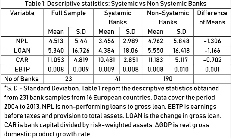
Table 1: Descriptive statistics: Systemic vs Non Systemic Banks
Variable Full Sample Systemic Banks
Non-Systemic Banks
Difference of Means Mean S.D Mean S.D Mean S.D
NPL 4.513 5.44 3.456 2.989 4.762 5.848 -1.306 LOAN 5.340 16.726 4.384 18.06 5.550 16.418 -1.166 CAR 11.053 4.819 10.481 2.851 11.183 5.117 -0.702 EBTP 0.008 0.009 0.009 0.008 0.008 0.010 0.001 No of Banks 23 41 190
*S. D - Standard Deviation. Table 1 report the descriptive statistics obtained from 231 bank samples from 16 European countries. Data cover the period 2004 to 2013. NPL is non-performing loans to gross loan. EBTP is earnings before taxes and provision to total assets. LOAN is the change in gross loan. CAR is bank capital divided by risk-weighted assets. ΔGDP is real gross domestic product growth rate.
Table 2 A and B reports the Pearson correlation coefficients and the associated p-values. Table 2a reports the correlation results for systemic banks. NPLs are not significantly correlated with EBTP. LOAN is significant and negatively correlated with NPLs for systemic banks, implying that systemic banks that increase loan supply experience fewer non-performing loans. CAR is significant and positively correlated with NPLs for systemic banks, implying that well-capitalised systemic banks experience higher problem loans. ∆GDP is negative and significantly correlated with NPLs, implying that problem loans are higher during bad times.
2A: Correlation for Systemic Banks
Table 2a report the correlation matrix for systemic banks. All bank level variables remain as previously defined. ***, ** and * represent significance at the 1%, 5% and 10% level, respectively. P-values are reported in parentheses.
Variable NPL LOAN ΔGDP EBTP CAR NPL 1.000
LOAN -0.372*** 1.000 (0.000)
ΔGDP -0.245*** 0.321*** 1.000 (0.000) (0.000)
EBTP 0.009 0.262*** -0.012 1.000 (0.893) (0.000) (0.862)
CAR 0.187*** -0.394*** -0.253*** -0.335*** 1.000 (0.005) (0.000) (0.000) (0.000)
Table 2B: Correlation for Non-Systemic Banks
Table 2a report the correlation matrix for non G-SIBs. All bank level variables remain as previously defined. ***, ** and * represent significance at the 1%, 5% and 10% level, respectively. P-values are reported in parentheses.
Variable NPL LOAN ΔGDP EBTP CAR NPL 1.000
LOAN -0.221*** 1.000 (0.000)
ΔGDP -0.279*** 0.234*** 1.000 (0.000) (0.000)
EBTP -0.032 0.246*** 0.144*** 1.000 (0.334) (0.000) (0.000)
5.2. Regression Result
5.2.1. Full Sample Analysis
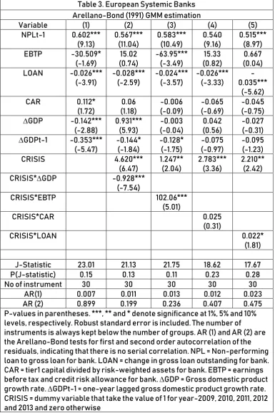
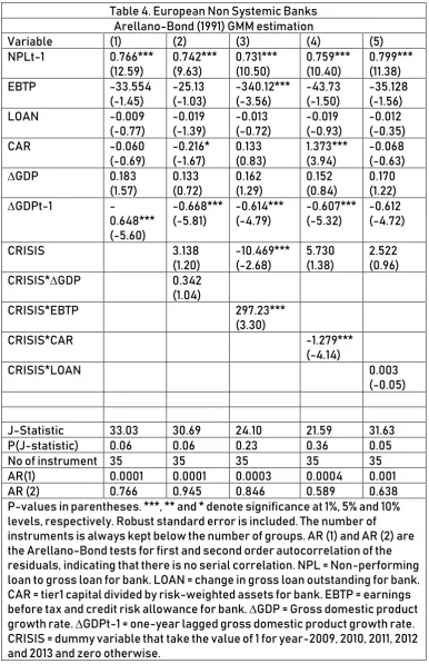
Column 1 of Table 3 and 4 report the dynamic (Arellano-Bond) regression estimations for systemic banks and non-systemic banks. ∆GDP coefficient is negatively significant, implying that systemic banks witness fewer NPLs during economic booms. But, the result is not significant for non-systemic banks. This finding is similar with the result of Glen and Mondragón-Vélez (2011) and Nkusu (2011) who show a link between non-performing loan and ∆GDP. The lagged GDP growth coefficient is negatively significant for both systemic and non-systemic banks, indicating that lagged GDP growth is inversely and significantly associated with growth of NPLs for both banks. This implies that banks’ asset quality deteriorates with a lag in response to negative economic growth possibly due to the difficulty of debtors to meet their obligation during bad economic times. The earnings coefficient (EBTP) reports a negative sign for both banks although the result is weakly significant for systemic banks and insignificant for non-systemic banks. This implies that NPLs are likely to impair the earnings of systemic banks than non-systemic European banks, however, the results do not show a strong link between NPLs and earnings before loan loss allowance (EBTP). Also, loan growth (LOAN) has a negative and significant impact on the non-performing loans of systemic banks. This suggest that systemic banks lend to less-risky borrowers, which leads to lower NPLs, and imply that systemic banks probably have a strong and prudent credit risk management system compared to non-systemic banks. Similarly, a negative relationship between NPLs and LOAN is observed for non-systemic banks but this relationship is insignificant. Finally, the CAR coefficient is positive and significant for systemic banks but is insignificant for non-systemic banks, indicating that systemic banks keep higher regulatory capital when they expect higher NPLs.
5.2.2. Behaviour of NPLs after the global financial crisis
Here, I introduce the ‘POST’ dummy variable that take the value ‘1’ for the post-financial crisis
Table 3. European Systemic Banks
Arellano-Bond (1991) GMM estimation
Variable (1) (2) (3) (4) (5) NPLt-1 0.602***
(9.13) 0.567*** (11.04) 0.583*** (10.49) 0.540 (9.16) 0.515*** (8.97) EBTP -30.509*
(-1.69) 15.02 (0.74) -63.95*** (-3.49) 15.33 (0.82) 0.667 (0.04) LOAN -0.026***
(-3.91) -0.028*** (-2.59) -0.024*** (-3.57) -0.026*** (-3.33) -0.035*** (-5.62) CAR 0.112*
(1.72) 0.06 (1.18) -0.006 (-0.09) -0.065 (-0.69) -0.045 (-0.75) ∆GDP -0.142***
(-2.88) 0.931*** (5.93) -0.003 (-0.04) 0.042 (0.56) -0.027 (-0.31) ∆GDPt-1 -0.353***
(-5.47) -0.144* (-1.84) -0.128* (-1.75) -0.075 (-0.97) -0.095 (-1.23) CRISIS 4.620***
(6.47) 1.247** (2.04) 2.783*** (3.36) 2.210** (2.42) CRISIS*∆GDP -0.928***
(-7.54)
CRISIS*EBTP 102.06*** (5.01)
CRISIS*CAR 0.025
(0.31)
CRISIS*LOAN 0.022*
(1.81)
J-Statistic 23.01 21.13 21.75 18.62 17.67 P(J-statistic) 0.15 0.13 0.11 0.23 0.28 No of instrument 30 30 30 30 30
AR(1) 0.007 0.011 0.013 0.012 0.023 AR (2) 0.899 0.199 0.236 0.407 0.475 P-values in parentheses. ***, ** and * denote significance at 1%, 5% and 10% levels, respectively. Robust standard error is included. The number of
Table 4. European Non Systemic Banks
Arellano-Bond (1991) GMM estimation
Variable (1) (2) (3) (4) (5) NPLt-1 0.766***
(12.59) 0.742*** (9.63) 0.731*** (10.50) 0.759*** (10.40) 0.799*** (11.38) EBTP -33.554
(-1.45) -25.13 (-1.03) -340.12*** (-3.56) -43.73 (-1.50) -35.128 (-1.56) LOAN -0.009
(-0.77) -0.019 (-1.39) -0.013 (-0.72) -0.019 (-0.93) -0.012 (-0.35) CAR -0.060
(-0.69) -0.216* (-1.67) 0.133 (0.83) 1.373*** (3.94) -0.068 (-0.63) ∆GDP 0.183
(1.57) 0.133 (0.72) 0.162 (1.29) 0.152 (0.84) 0.170 (1.22) ∆GDPt-1
-0.648*** (-5.60) -0.668*** (-5.81) -0.614*** (-4.79) -0.607*** (-5.32) -0.612 (-4.72)
CRISIS 3.138
(1.20) -10.469*** (-2.68) 5.730 (1.38) 2.522 (0.96) CRISIS*∆GDP 0.342
(1.04)
CRISIS*EBTP 297.23*** (3.30)
CRISIS*CAR -1.279***
(-4.14)
CRISIS*LOAN 0.003
(-0.05)
J-Statistic 33.03 30.69 24.10 21.59 31.63 P(J-statistic) 0.06 0.06 0.23 0.36 0.05 No of instrument 35 35 35 35 35 AR(1) 0.0001 0.0001 0.0003 0.0004 0.001 AR (2) 0.766 0.945 0.846 0.589 0.638 P-values in parentheses. ***, ** and * denote significance at 1%, 5% and 10% levels, respectively. Robust standard error is included. The number of
5.3. Further Analyses
5.3.1. Size of Earnings Effect
Next, I analyse the behaviour of NPLs when banks have high profits or high loses. To test whether non-performing loans are significantly associated with earnings when both banks expect losses or high earnings, the NEG and POS dummy variables are interacted with EBTP. The result is reported in Column 1 and 5 of Table 5. The results show that NPLs are positive and strongly linked with EBTP when both banks are more profitable. This implies that, in the face of high non-performing loans (i.e., declining asset quality), both banks remain profitable (before adjustment for provisions) while column 2 and 6 show that NPLs are fewer for non-systemic banks when they experience higher losses, and insignificant for systemic banks.
5.3.2. Higher Regulatory Capital Effect
Next, I analyse the behaviour of NPLs when banks have sufficient (regulatory) capital. To test whether bank non-performing loans is significantly associated with Tier 1 capital when the banks have sufficient Tier 1 regulatory capital ratio (i.e., above 8% tier 1 capital), WELL dummy variable is interacted with the CAR variable. Column 3 report a negative relationship between NPLs and WELL*CAR for systemic banks but this relationship is not significant for systemic banks. One possible explanation for the weak relationship could be due to the fact that Tier 1 capital for systemic banks may be used more extensively to mitigate other risks (such as market risk, interest rate etc.) rather than to mitigate only credit risk. On the other hand, Column 7 report a positive and significant relationship between NPLs and above-8% Tier 1 capital for non-systemic banks. This indicates that non-systemic banks with sufficient regulatory capital experience higher NPLs.
5.3.3. Excess Credit Supply Effect
Table 5 - Sensitivity Analysis - Regression
Systemic Banks Non-systemic
Variable 1 2 3 4 5 6 7 8 NPLt-1 0.583***
(7.56) 0.586*** (8.49) 0.701*** (9.62) 0.743*** (9.68) 0.794*** (12.48) 0.863* (1.87) 0.697*** (8.77) 0.994*** (11.13) EBTP -163.78***
(-4.03) -5.256 (-0.25) -38.220 (-1.47) -56.36** (-2.01) -85.396*** (-3.59) 184.42*** (2.52) -6.199 (-0.16) -69.024 (-1.14)
LOAN -0.035*** (-4.97) -0.020*** (-2.73) -0.019*** (-2.63) -0.009 (-0.56) 0.023 (1.01) -0.023 (-1.05) CAR 0.075
(1.27) 0.126 (1.24) 1.035 (1.29) 0.284** (2.42) -0.062 (-0.55) -0.099 (-0.85) -0.785* (-1.89) 0.120 (1.29)
∆GDP -0.158** (-2.55) -0.160*** (-2.64) -0.217*** (-3.38) -0.006 (-0.06) 0.409** (2.49) 0.038 (0.22) 0.669*** (3.51) -0.310*** (-4.20)
∆GDPt-1 -0.348*** (-5.56) -0.275*** (-4.63) -0.287** (-2.07) -0.159*** (-2.71) -0.568*** (-4.08) -0.504*** (-3.25) -0.642*** (-4.93) -0.076 (-0.63) POS 0.316
(0.85)
-3.503*** (-3.25) POS*EBTP 104.65***
(2.60)
350.23*** (4.22) NEG 0.856*
(1.76)
7.805*** (2.78) NEG*EBTP -55.486
(-0.47)
-184.61** (-2.36)
WELL 3.972
(0.76)
-1.576 (-0.69) WELL*CAR -0.851
(-1.08)
0.668* (1.85) In(LOAN) -0.082*
(-1.80)
0.243* (1.83)
J-Statistic 19.19 23.27 16.96 16.32 21.88 18.11 22.01 18.80 P(J-Stat) 0.21 0.08 0.32 0.29 0.35 0.580 0.34 0.65
No of instrument
30 30 30 27 35 35 35 35
AR(1) 0.015 0.007 0.008 0.04 0.0001 0.004 0.0002 0.0005 AR (2) 0.578 0.418 0.055 0.852 0.639 0.687 0.796 0.130 P-values in parentheses. ***, ** and * denote significance at 1%, 5% and 10% levels, respectively. Robust standard error is included. The number of instruments is always kept below the number of groups. AR (1) and AR (2) are the Arellano-Bond tests for first and second order autocorrelation of the residuals, indicating that there is no serial correlation. NPL = Non-performing loan to gross loan for bank i at time t. LOAN = change in gross loan outstanding. CAR = tier1 capital divided by risk-weighted assets for bank i at time t. EBTP = earnings before tax and credit risk allowance. ∆GDP = Gross domestic product growth rate.
5. Concluding Remarks
The distinction between GSIBs and non GSIBs is driven by policy reasons. This study adopts this policy classification to investigate the relationship between nonperforming loans (NPLs) and the economic cycle for European systemic and non-systemic banks after controlling for earnings before loan loss allowance, bank lending, and bank tier 1 capital ratios. The findings reveal that systemic banks have fewer non-performing loans during economic booms. Also, increased lending is associated with few NPL in systemic banks, implying that systemic banks have a strong and prudent credit risk mitigation process that mitigates or reduce the risks in their loan portfolio while higher lending is associated with higher NPLs for non-systemic banks. Systemic banks keep higher regulatory capital when they expect higher NPLs while non-systemic banks that exceed regulatory capital requirements experience higher NPLs. Non-systemic banks have fewer NPLs when they experience higher losses. Finally, more profitable banks witness higher NPLs regardless of whether they are systemic or non-systemic banks.
The implication of the findings is that national supervisors need to strengthen the micro-prudential supervision of systemic banks in their countries to reduce abnormal NPLs to the lowest possible. To achieve this, supervisors can use a combination of micro- and macro-prudential policies for banking supervision and regulation. Also, the observation that increased lending is associated with few NPLs in systemic banks but not in non-systemic banks is interesting. This calls for increased regulatory oversight on the lending practices of European banks by bank supervisors. However, bank supervisors must also exercise caution and understand that excessive focus on the supervision of systemic banks can have unintended consequences if credit risks in non-systemic banks are not monitored properly by national supervisors.
Reference
Acharya, V., Pedersen, L., Philippe, T., and Richardson, M. (2010). Measuring systemic risk. Technical report, Department of Finance, NYU
Adrian, Tobias, and Markus K. Brunnermeier, 2011, CoVaR, Staff Reports 348, Federal Reserve Bank of New York.
Aiyar, M. S., Bergthaler, Garrido, Monaghan, M. D., et al (2015). A strategy for resolving Europe's problem loans. International Monetary Fund. Available at: https://www.imf.org/external/pubs/ft/sdn/2015/sdn1519.pdf Accessed on 12 January, 2019.
Allen, L., Bali, T. G., & Tang, Y. (2012). Does systemic risk in the financial sector predict future economic downturns? The Review of Financial Studies, 25(10), 3000-3036.
Arellano, M., & Bond, S. (1991). Some tests of specification for panel data: Monte Carlo evidence and an application to employment equations. The review of economic studies, 58(2), 277-297.
Banulescu, G. D., & Dumitrescu, E. I. (2015). Which are the SIFIs? A Component Expected Shortfall approach to systemic risk. Journal of Banking & Finance, 50, 575-588.
Basel, II. (2004). International convergence of capital measurement and capital standards: a revised framework. Bank for international settlements.
Beck, R., Jakubik, P., & Piloiu, A. (2013). Non-performing loans: What matters in addition to the economic cycle? (February 11, 2013). ECB Working Paper No. 1515. Available at SSRN:
https://ssrn.com/abstract=2214971
Beck, R., Jakubik, P., & Piloiu, A. (2013). Non-performing loans: What matters in addition to the economic cycle?
Besanko, D., & Kanatas, G. (1996). The regulation of bank capital: Do capital standards promote bank safety? Journal of financial intermediation, 5(2), 160-183.
Benink, H., & Wihlborg, C. (2002). The new Basel capital accord: making it effective with stronger market discipline. European Financial Management, 8(1), 103-115.
Black, Lamont, Ricardo Correa, Xin Huang, and Hao Zhou, 2013, The Systemic Risk of European Banks during the Financial and Sovereign Debt Crises, Working Paper.
Bleck, A. (2018). Regulating bank leverage. Journal of Financial Economic Policy, 10(2), 264-274.
Brownlees, C. T., & Engle, R. (2012). Volatility, correlation and tails for systemic risk measurement. Available at SSRN, 1611229.
Carey, M. (1998). Credit risk in private debt portfolios. The Journal of Finance, 53(4), 1363-1387.
Drehmann (2005) A Market Based Macro Stress Test for the Corporate Credit Exposures of UK Banks. An unpublished article, Bank of England, March 2005.
Espinoza, R. A., & Prasad, A. (2010). Nonperforming loans in the GCC banking system and their macroeconomic effects (No. 10-224). International Monetary Fund.
European Commission, EC, (2018). Proposal for a regulation of the European parliament and of the council amending regulation (EU) No 575/2013 as regards minimum loss coverage for non-performing exposure: Impact assessment. Accessed on: 5th June, 2018. Available at:
European Commission, 2013, Regulation No 575/2013 on prudential requirements for credit institutions and investment firms (CRR). http://eur-lex.europa.eu/legal-content/EN/TXT/?uri=celex:32013R0575
European Commission, 2014, Proposal for a regulation on structural measures improving the resilience of EU credit institutions, COM(2014) 043 final. http://eur-lex.europa.eu/legal-content/EN/ALL/?uri=CELEX:52014PC0043
Fofack, H. L. (2005). Nonperforming loans in Sub-Saharan Africa: causal analysis and macroeconomic implications. The World Bank.
Glen, J., & Mondragón-Vélez, C. (2011). Business cycle effects on commercial bank loan portfolio performance in developing economies. Review of Development Finance, 1(2), 150-165.
Huang, Xin, Hao Zhou, and Haibin Zhu, 2009, A Framework for Assessing the Systemic Risk of Major Financial Institutions, Journal of Banking and Finance, Vol. 33, No. 11, 2036- 2049.
Huang, Xin, Hao Zhou, and Haibin Zhu, 2012, Systemic Risk Contributions, Journal of Financial Services Research, Vol. 42, No. 1-2, 55-83
Karimalis, E. N., & Nomikos, N. K. (2018). Measuring systemic risk in the European banking sector: A Copula CoVaR approach. The European Journal of Finance, 24(11), 944-975.
Klein, N. (2013). Non-performing loans in CESEE: Determinants and impact on macroeconomic performance (No. 13-72). International Monetary Fund.
Louzis, D. P., Vouldis, A. T., & Metaxas, V. L. (2012). Macroeconomic and bank-specific determinants of non-performing loans in Greece: A comparative study of mortgage, business and consumer loan portfolios. Journal of Banking & Finance, 36(4), 1012-1027.
Nkusu, M. M. (2011). Nonperforming loans and macrofinancial vulnerabilities in advanced economies (No. 11-161). International Monetary Fund.
Ozili, P. K. (2019). Non-performing loans and financial development: new evidence. The Journal of Risk Finance, 20(1), 59-81.
Pesaran, M.H., 2006. Estimation and inference in large heterogeneous panel with a multifactor error structure. Econometrica 74 (4), 967–1012.
Pesola (2005) Banking fragility and distress: An econometric study of macroeconomic determinants. Bank of Finland Research Discussion Papers, No. 13.
Quagliariello, M. (2007). Banks’ riskiness over the business cycle: a panel analysis on Italian
intermediaries. Applied Financial Economics, 17(2), 119-138.
Ruckes, M. (2004). Bank competition and credit standards. Review of Financial Studies, 17(4), 1073-1102.
Salas, V., & Saurina, J. (2002). Credit risk in two institutional regimes: Spanish commercial and savings banks. Journal of Financial Services Research, 22(3), 203-224.
Shrieves, R. E., & Dahl, D. (1992). The relationship between risk and capital in commercial banks. Journal of Banking & Finance, 16(2), 439-457.
Wezel, T., Canta, M., & Luy, M. (2014). A practical example of the nonperforming loans projection approach to stress testing. A Guide to IMF Stress Testing: Methods and Models, 473-483.
Appendix
A1: Summary of Sample Distribution
Country G-SIBs Non G-SIBs # Banks United Kingdom 13 22 35 Germany 2 24 26
Ireland 1 9 10
Luxembourg 2 5 7
Norway 1 6 7
Denmark 1 10 11
Finland 1 3 4
Greece 0 4 4
Portugal 2 4 6
Belgium 1 9 10
Netherland 3 9 12
Sweden 2 9 11
Spain 2 8 10
France 7 28 35
Italy 2 27 29
Austria 1 13 14