Munich Personal RePEc Archive
Weather Shocks
Gallic, Ewen and Vermandel, Gauthier
Aix-Marseille Univ., CNRS, EHESS, Centrale Marseille, AMSE,
Universités Paris-Dauphine PSL, France Stratégie
26 August 2017
Online at
https://mpra.ub.uni-muenchen.de/93905/
Weather Shocks
∗Ewen Gallica and Gauthier Vermandel†b,c
aAix-Marseille Univ., CNRS, EHESS, Centrale Marseille, AMSE. bParis-Dauphine and PSL Research Universities
cFrance Strat´egie, Services du Premier Ministre
May 13, 2019
Abstract
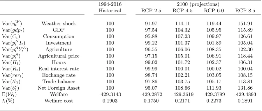
How much do weather shocks matter? The literature addresses this question in two isolated ways: either by looking at long-term effects through the prism of theoretical models, or by focusing on short-term effects using empirical analysis. We propose a framework to bring together both the short and long-term effects through the lens of an estimated DSGE model with a weather-dependent agricultural sector. The model is estimated using Bayesian methods and quarterly data for New Zealand using the weather as an observable variable. In the short-run, our analysis underlines the key role of weather as a driver of business cycles over the sample period. An adverse weather shock generates a recession, boosts the non-agricultural sector and entails a domestic currency depreciation. Taking a long-term perspective, a welfare analysis reveals that weather shocks are not a free lunch: the welfare cost of weather is currently estimated at 0.19% of permanent consumption. Climate change critically increases the variability of key macroeconomic variables (such as GDP, agricultural output or the real exchange rate) resulting in a higher welfare cost peaking to 0.29% in the worst case scenario.
Keywords : Agriculture, Business Cycles, Climate Change, Weather Shocks
JEL classification: C13, E32, Q54
∗We thank St´ephane Adjemian, Catherine Benjamin, Paul Chavas, Fran¸cois Gourio, Alexandre
Jean-neret, Michel Juillard, Fr´ed´eric Karam´e, Robert Kollmann, Olivier L’Haridon, Fran¸cois Langot, Michel Nor-mandin, Jean-Christophe Poutineau, Katheline Schubert, and Christophe Tavera for their comments. We thank participants at the Climate Economic Chair Workshop at Dauphine, Dynare-ECB conference, T2M in Lisbon, the CEF in New-York, the SURED 2016 conference, the French Economic Association annual meeting in Nancy, the INRA workshop in Rennes, the GDRE conference in Clermont-Ferrand, the ETEPP-CNRS 2016 conference in Aussois, IMAC Workshop in Rennes, and seminars at the University of Caen, the University of Rennes 1, Paris-Dauphine, Utrecht University, and the University of Maine. We remain responsible for any errors and omissions.
†Corresponding author:
1
Introduction
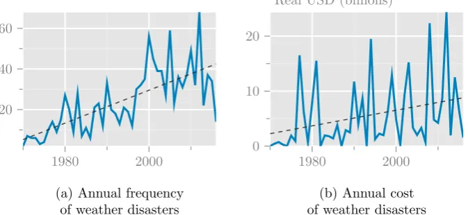
Among the many shocks and disturbances driving the business cycles, the weather has received little attention as a serious source of business cycles in modern macroeconomic models. Yet over the last 40 years, heat waves and droughts have been causing significant damages at global level peaking to a total value of US$25 billion in 2014, as documented inFigure 1. Both the frequency and the intensity of these adverse events tend to follow an upward trend, suggesting that the weather is likely to become a more frequent source of business cycles in the coming years. This growing source of macroeconomic fluctuations, also referred to as weather shocks, is emerging as one of the most important facets of global warming, in particular for agricultural-based countries. In such economies, the weather generates detrimental fluctuations in the agricultural sector that can spread to the rest of the economy.
1980 2000 20
40 60
(a) Annual frequency of weather disasters
1980 2000 0
10 20
Real USD (billions)
(b) Annual cost of weather disasters
[image:3.595.114.451.252.407.2]Note: Data are taken from EM-DAT; IMF, World Economic Outlook database and set in real terms using the US GDP deflator.
Figure 1: Global frequency and impact of weather shocks (droughts and heat waves) between 1970 and 2016.
If long-run effects of the weather, i.e., climate effects are already well documented in the literature,1 many uncertainties remain regarding the short-run aspects in terms of propagation,
supply-side transmission channels and the potential welfare costs. More importantly, most of this literature considers the change in climate statistics as a trend phenomenon (e.g.,Nordhaus and Yang, 1996; Nordhaus, 2018b, 1991), leaving the role of weather fluctuations and their underlying welfare costs as second order issues. In this article, we argue that weather driven business cycles are not a benign facet of climate change.
Contributions. The aim of this article is therefore to fill the gap by making three main contributions to address this question. The first contribution concerns the engineering of an aggregate measure of the weather. Unlike TFP shocks which are not observable, the time-varying productivity of agricultural lands is measurable from soil moisture observations.2 In this paper, we build a weather index at a macro level from soil moisture deficits observations
1SeeAcevedo et al.(2017) for a survey on weather shocks,Nordhaus(2018a) for a summary of the evolution
of the DICE model over the three decades, andDeschenes and Greenstone(2007) for an assessment of long term effects of climate change on agricultural output.
2Therefore in the rest of the article, we refer to these exogenous changes in land productivity as weather
that captures unsatisfactory levels of agriculture productivity for New Zealand.3 A second
contribution lies in the documentation of the transmission mechanisms of the weather. Through the lens of a Vector Auto-Regressive (VAR) model, we gauge the quantitative interaction of the weather with seven macroeconomic time series of New Zealand. Following a shock to the weather equation in the VAR, we document the transmission mechanism of the weather in a small-open economy environment. A third contribution concerns the building of a macroeconomic model with a time-varying weather. We enrich a Dynamic Stochastic General Equilibrium (DSGE) model with a tractable weather-dependent agricultural sector. Entrepreneurs involved in the agricultural sector (i.e., farmers) are endowed with a land. The productivity of that land is endogenously determined by both economic and weather conditions. Farmers face unanticipated weather shocks affecting the efficiency of their land over the business cycles. The model is estimated through Bayesian techniques with the same sample as the VAR model to provide an alternative theoretical representation of the data. In addition to its empirical relevance, the estimated DSGE model is amenable for counterfactual experiments to assess the quantitative implications of climate change on the business cycles of an economy.
We get three main results from the aforementioned methodology. First, both the VAR and the DSGE models document the transmission of a weather shock – more specifically a drought – through a large and persistent contraction of agricultural production, accompanied by a decline in consumption, investment and a rise in hours worked. At an international level, a weather shock causes current account deficits and a depreciation of the domestic currency. The weather shock thus shares similar dynamic patterns with a sectoral TFP shock. Second, we find that weather shocks play a non-trivial role in driving the business cycles of New Zealand. On the one hand, the inclusion of weather-driven business cycles strikingly improves the statistical performance of the model. On the other hand, the weather drives an important fraction of the unconditional variance, in particular for GDP, consumption and agricultural output. The resulting consequence is a high welfare cost of business cycles induced by weather shocks. In particular, we find that households would be willing to give up 0.19% of their unconditional consumption to rule out weather shocks, which is remarkably high with respect to other sources of disturbances in our model. A third result concerns an original counterfactual analysis on climate change. We increase the volatility of weather shocks in accordance with IPCC(2014)’s climate change projections for 2100, and evaluate how these structural changes in the distribu-tion of weather shocks affect macroeconomic volatility. We find that climate change critically increases the variability of key macroeconomic variables, such as GDP, agricultural output or the real exchange rate. The corollary of this structural change is an increase of the welfare cost of weather driven business cycles peaking up to 0.29% in the worst-case climate change scenario. To the best of our knowledge, this article is the first to use full-information methods to estimate a theoretical model with the weather as an observable variable to gauge the current and future cost of the weather at a business cycle frequency.
Related literature. Our work contributes to the literature that connects the macroe-conomy with the weather through the lens of theoretical models. This literature is mainly dominated by integrated assessment models (IAMs) pioneered by Nordhaus (1991). In a nut-shell, this literature links climate and economic activity through a damage function that lies in the firms’ production technology. Thus, an increase in temperatures due to greenhouse gas emissions causes higher damages to aggregate production. However, this literature focuses on
3We use New Zealand data for two reasons. First, New Zealand has faced many weather shocks, in particular
very long run effects of climate change through deterministic simulations.4 We build on this
ap-proach by using a damage function that connects the weather to the farmers’ land productivity. We complement the IAMs literature by tackling the short-term dimension of the weather, and evaluate their social costs in a context of climate change.
Another strand of the literature employs empirical models to examine the short-run effects of the weather on economic activity. In particular, some authors focus on the relationship be-tween temperatures and productivity. Dell et al. (2012) show that high temperatures have a detrimental effect on economic growth, but only in poor countries. These results are contrasted by the empirical study of Burke et al. (2015) which shows that the relationship between high temperatures and productivity is non-linear, for both poor and rich countries. The studies of Acevedo et al.(2017) andMejia et al.(2018), conducted on larger samples, confirm these results. In addition, Fomby et al.(2013) show that in the case of developed countries, droughts have a negative effect on growth, in particular for the agricultural sector. Our analytical framework builds on these studies to model how climate can affect the economic activity. We focus on the agricultural sector, making productivity in this sector dependent on weather shocks. We also rely on the results of empirical studies that focus more on the weather and the economy at business cycle frequency. For example,Buckle et al.(2007) andKamber et al. (2013) underline the importance of weather variations as a source of aggregate fluctuations, along with interna-tional trade price shocks, using a structural VAR model for New Zealand. Bloor and Matheson (2010) find evidence of the importance of the weather, more particularly the occurrence of El Ni˜no events, on agricultural production and total output in New Zealand. Cashin et al.(2017) also investigate the effects of El Ni˜no on the world economy, using a country-by-country analy-sis. More specifically, they find evidence of negative effects of an El Ni˜no shock on real output growth in New Zealand. Finally, in a recent study,Donadelli et al.(2017) propose a framework related to ours. In a real business cycle model, they introduce temperature levels as an explana-tory factor of productivity for the US economy. In their model, productivity is affected by the unpredictable component of temperatures. Their results show that a one-standard deviation temperature shock causes a 1.4 percentage point decrease in productivity growth. The authors emphasize the importance of temperature shocks regarding welfare costs. Our article comple-ments this study by taking a theoretical model to the data, instead of limiting the analysis to a calibration exercise. In addition, our measure of the weather is not limited to tempera-tures, as our weather index also includes the role of rainfalls and its possible interaction with temperatures through evapotranspiration.
The remainder of this article is organized as follows: Section 2 provides some empirical evidences through the lens of a VAR model regarding the impact of weather shocks on macroe-conomic variables. Section 3 sketches the Dynamic Stochastic General Equilibrium model. Section 4 presents the estimation of the DSGE model. Section 5 provides evidence on the importance of introducing weather shocks in the model. Section 6 discusses the propagation of a weather shock, assesses the consequences of a drought and its implication in terms of business cycles statistics, and presents the historical variance decomposition of supply of the economy. Section 7 conducts a sensitivity analysis to illustrate how the parameters of the weather-dependent agricultural sector affect our results. Section 8 provides a quantitative as-sessment of the implications of weather shocks under different climate projection scenarios for aggregate fluctuations, and estimates the welfare cost of weather shocks. Section 9 concludes.
4A notable exception, fromCai and Lontzek(2019), expands the scope of IAMs by adding uncertainties and
2
Business Cycle Evidence
How do we measure the weather? In most of the models in environmental economics, weather and climate measurements are solely based on temperature records. In agricultural economics these measures are often supplemented by rainfall observations in order to characterize agricul-tural returns patterns. In this paper, the weather is measured through soil moisture deficits. Soil moisture deficits depict the balance ratio between rainfalls and temperatures. Rainfalls typically boost the productivity of the land by favoring crop growth, and conversely the evap-otranspiration process induced by higher temperatures reduces land productivity.5 Based on
observations of soil moisture deficits, we build a macroeconomic index6 that aims at providing an accurate measure of land productivity in New Zealand. A graphical representation of this index is provided in Figure 2. By construction, the index values range from -4 to +4, where positive values indicate a soil moisture deficit, while negative ones indicate an excess of moisture.
1998 2000 2002 2004 2006 2008 2010 2012 2014 2016
−2
−1.5
−1
−0.5 0 0.5 1 1.5 2
[image:6.595.163.423.265.410.2]Soil moisture deficits index Top 10% severe droughts threshold
Figure 2: Weather index measuring soil moisture deficits in New Zealand.
As shown inFigure 2, New Zealand has experienced cyclical changes in its soil water deficits index over the last two decades, oscillating between periods of high volumetric water content in soils and periods of droughts. Assuming a normal distribution of the weather, the 10th percent of the most severe episodes can be inferred directly from the time series when the soil moisture deficits index peaks above 1. In the same way as for NBER recessions, the index allows to easily date and monitor severe weather events which are very likely to be costly for the agricultural sector as shown byKamber et al.(2013) andMejia et al. (2018). In recent years, New Zealand has undergone numerous episodes of severe droughts of various intensities that have disrupted its economy to a greater or lesser extent, most notably in 2007, 2010, 2013 and 2015.
What is the supply-side adjustment of New Zealand following a severe drought? A pre-liminary assessment of these extreme events on the sectoral reallocation is performed through the examinations of changes in the relative share of each sector in the total production of New Zealand. Figure 3 reports these changes in the shares of agriculture, primary, secondary, and tertiary sectors in total activity, two quarters before and four quarters after the four most severe droughts. For convenience, each sector’s share of the total activity is normalized to 100 at the time of the drought. Each line corresponds to a drought episode reported by the index at hand. After a drought shock, the share of the agricultural sector in total output declines substantially although temporarily. A similar pattern is observed for the primary sector, although the magni-tude of the reaction is naturally not as important as for agriculture because the primary sector includes mining and fishing which are less sensitive to the weather. Regarding the secondary
5SeeDoorenbos and Kassam(1979) andNarasimhan and Srinivasan(2005) for a analysis of soil moisture on
crop yields.
Secondary Sector Tertiary Sector
Agriculture Primary Sector
-2 0 2 4 -2 0 2 4
-2 0 2 4 -2 0 2 4
96 100 104 108
99.5 100.0 100.5 101.0 90
100 110
97 98 99 100 101
Drought 2007:Q2 2010:Q2 2013:Q1 2015:Q4
[image:7.595.90.494.71.272.2]Notes: The lines show the evolution before and after a drought for each sector’s share in total production, after normalizing the sector’s share to 100 at the time of the drought.
Figure 3: Sectoral re-allocations following severe weather shocks.
sector, the result is unclear suggesting that there is no salient effects. As for the tertiary sector, it tends to experience a relative expansion, in accordance with Mejia et al. (2018), suggesting that weather shocks possibly generate positive spillover effects.
Correlation T-Stat P-value 95% Confidence interval Agriculture Only -0.31 -2.99 0.00 [−0.48,−0.10] Primary Sector -0.25 -2.41 0.02 [−0.44,−0.04] Secondary Sector -0.10 -0.91 0.37 [−0.30,0.11] Tertiary Sector 0.39 3.90 0.00 [0.19,0.55]
Notes: The significance of correlations is tested using the Pearson test.
Table 1: Correlations of Sectoral GDP with the weather index.
To complete the assessment, we compute correlations between the time series of the weather and the relative share of different sectors used in the previous figure. Table 1also corroborates the presence of possible sectoral adjustments. In particular, the share of the agricultural sector is negatively correlated with the weather index, as is, to a lesser extent, the GDP of the primary and secondary sectors. On the other hand, the activity of the tertiary sector is positively correlated with the drought measure.
To investigate further the interactions between the weather and other standard macroeco-nomic time series, a vector autoregressive model is employed. A few constraints on the VAR’s equations are necessary to portray New Zealand’s specific situation: (i) we impose an exogenous weather (i.e., the weather is not Granger caused by any other variable),7 (ii) we force domestic
7As the historical data only cover a restricted period of time, we assume that human activities do not
[image:7.595.120.472.392.458.2]variables to have no effect on foreign variables asCushman and Zha(1997).8 The VAR includes
8 observable variables. Six of them represent the domestic block: GDP, agricultural produc-tion, consumpproduc-tion, investments, hours worked, and variations of the real effective exchange rate. The foreign block contains a measure of GDP for the rest of the world.9 All these variables are
taken in real terms and expressed in percentage deviations from a log-linear trend. In addition, the restricted VAR model is estimated with one lag, as suggested by both Hannan-Quinn and Schwarz criteria.
5 10 15 20
−0.3
−0.2
−0.1 0
GDP
5 10 15 20
−0.4
−0.3
−0.2
−0.1 0
Consumption
5 10 15 20
−2
−1 0
Agriculture
5 10 15 20
−1
−0.5 0 0.5
Investment
5 10 15 20 0
0.2 0.4
Hours
5 10 15 20
−0.6
−0.4
−0.2 0
Domestic ∆ RER
5 10 15 20
−0.5 0 0.5 1
Foreign GDP
5 10 15 20 0
0.2 0.4 0.6 0.8
Weather
VAR mean VAR mean±1 std
[image:8.595.72.513.169.355.2]Notes: The green dashed line is the Impulse Response Function. The gray band represents 68% error band obtained from the 250 bootstraps runs. The response horizon is in quarters. Time horizon is plotted on the x-axis while the percent deviation from the steady state is plotted on the y-axis.
Figure 4: VAR impulse response to a 1% weather shock (drought) in New Zealand.
To investigate the effects of an adverse weather shock, we examine the impulse responses to a one-standard-deviation of the drought variable. A lower triangular Choleski decomposition of the error variance-covariance matrix is used to derive the orthogonal impulse responses. The results are depicted inFigure 4, where each panel represents the response of one of the variables to a weather shock. Overall, a shock to the weather shock equation generates a contraction of New Zealand’s economy in the similar magnitude as Buckle et al. (2007): a rise in soil moisture deficits implies a 1.5% contraction of agricultural production, as already suggested by the two previous assessments. This depression in agriculture is simultaneously followed by a 0.3% decline in consumption and a 0.6% decline in investment. The adjustment of the labor market is naturally slower and materialize through a late rise in hours worked occurring 7 quarters after the realization of the weather shock, thus suggesting that the weather mimics the dynamic patterns of a TFP shock. The weather shock vanishes five periods after its realization, although its effects on the economy are strikingly very persistent, in particular for the labor market. This suggests the presence of an unusual propagation mechanism inherent to the weather which is to be taken into account in the modeling of the DSGE presented in the remainder of the article. More specifically, the presence of a slow adjustment effect will require a specific
8In particular, a first constraint concerns the small open economy nature of New Zealand with respect to its
trading partners. Letting New Zealand be the domestic country and NZ trading partners be the foreign country, we prevent both domestic shocks and variables to cause fluctuations on foreign variables. We followCushman and Zha(1997) and create an exogenous block for the variables from the rest of the world. We impose a second constraint on the VAR’s equations concerning the weather itself. In particular, exogeneity is also imposed for the weather variable, so that it can affect the domestic macroeconomic variables, and so that neither domestic nor foreign macroeconomic variables can affect the weather variable. More details are given in the paper’s online appendix.
9We use a weighted average of GDP for New Zealand’s top trading partners, namely Australia, Germany,
friction for the farmer problem.
3
The Model
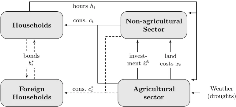
Our model is a two-sector, two-good economy in a small open economy setup with a flexible exchange rate regime.10 The home economy, i.e., New Zealand, is populated by households and firms. The latter operate in the agricultural and the non-agricultural sectors. Workers from the agricultural sector face unexpected weather conditions that affect the productivity of their land. Households consume both home and foreign varieties of goods, thus creating a trading channel adjusted by the real exchange rate. The general structure of the model is summarized inFigure 5. The remainder of this section presents the main components of the model.
Households
Foreign Households
Non-agricultural Sector
Agricultural sector
Weather (droughts)
cons.ct
cons.c∗
t
hoursht
land
costsxt
invest-mentiAt
[image:9.595.118.504.260.435.2]bonds b∗t
Figure 5: The theoretical model.
3.1 Agricultural Sector
The economy is populated by a unit massi∈[0,1] of infinite living and atomistic entrepreneurs. A fractionntof these entrepreneurs are operating in the agricultural sector while the remaining
fraction 1−nt operates in the non-agricultural sector. We allow any of the entrepreneurs to
switch from one sector to another assuming that the fixed portion of agricultural firms is subject to an exogenous shock: nt = n×εNt where εNt is a stochastic AR(1) process.11 The fraction
i∈[0, nt] of entrepreneurs operating in the agricultural sector is referred to as farmers.
To investigate the implications of variations of the weather as a source of aggregate fluctua-tions, a weather variable denotedεWt is introduced in the model. More specifically, this variable captures variations in soil moisture that affect the production process of agricultural goods. To be consistent with the VAR model, we assume that the aggregate drought index follows an autoregressive process with only one lag:
log(εWt ) =ρW log(εWt−1) +σWηWt , ηtW ∼ N(0,1), (1)
10Our small open economy setup includes two countries. The home country (here, New Zealand) participates
in international trade but is too small compared to its trading partners to cause aggregate fluctuations in world output, price and interest rates. The foreign country, representing most of the trading partners of the home country, is thus not affected by macroeconomic shocks from the home country, but its own macroeconomic developments affect the home country through the trade balance and the exchange rate.
11More specifically, theAR(1) shock is given by: log(εN
where ρW ∈[0,1) is the persistence of the weather shock and σW ≥ 0 its standard deviation.
In the model, shock processes are all normalized to one in the steady state so that a positive realization ofηWt – thus settingεWt above one – depicts a possibly prolonged episode of dryness that damages agricultural output. The stochastic nature of the model imposes that farmers are surprised by contemporaneous and future weather shocks. We do not consider the perspective of news shocks about the weather, as the usual forecast horizon for farmers about weather shocks lies between 1 and 15 days.12
The outcome of farmers’ activity in the agricultural sector encompasses a large variety of goods such as livestock, vegetables, plants, or trees. All of these agricultural goods typically require land, labor and physical capital as input be produced. The general practice in agricul-tural economics is to explicitly feature the input-output relationship by imposing a functional form on the technology of the agricultural sector.13 Among many possible functional forms,
the Cobb-Douglas production function has become popular in this economic field following the contribution of Mundlak (1961).14 We accordingly assume that agricultural output is Cobb-Douglas in land, physical capital inputs, and labor inputs:
yitA=Ω εWt ℓit−1 ωh
εZt kAit−1α κAhAit
1−αi1−ω
, (2)
where yAit is the production function of the intermediate agricultural good that combines an amount of land ℓit−1 (subject to the weather Ω εWt
through a function described later on), physical capital kAit−1, and labor demand hAit. Production is subject to an economy-wide tech-nology shock εZt following an AR(1) shock process affecting the two sectors. The parameter ω∈[0,1] is the elasticity of output to land,α∈[0,1] denotes the share of physical capital in the production process of agricultural goods, and κA >0 is a technology parameter endogenously
determined in the steady state. We include physical capital in the production technology, as, in developed countries the agricultural sector heavily relies on mechanization. Because of the delays in the settlement of physical capital and land, these two variables naturally embody “time to build” features `a la Kydland and Prescott (1982).
Each farmer owns a land ℓit that is subject to changes depending both on economic and
meteorological conditions. During the production process of agricultural goods betweent−1 and t, landℓit−1is subject to the unexpected realization of the weatherεWt . Agricultural production
is tied up with exogenous weather conditions through a damage function Ω(·) in the same spirit as the Integrated Assessment Models literature pioneered by Nordhaus (1991). We opt for a simple functional form for this damage function:15
Ω εWt = εWt −θ, (3)
whereθdetermines elasticity of land productivity with respect to the weather. Imposing θ= 0
12For example, in New Zealand the NIWA provides forecast services to farmers about weather shocks at a high
frequency level (1 or 2 days ahead), medium frequency level (6 days ahead) and probabilistic forecast out of fifteen days.
13SeeChavas et al.(2010) for a survey about the building of theoretical models in agricultural economics over
the last century.
14We refer toMundlak(2001) for discussions of related conceptual issues and empirical applications regarding
the functional forms of agricultural production. In an alternative version of our model based on a CES agricultural production function, the fit of the DSGE model is not improved, and the identification of the CES parameter is weak.
15The literature on IAMs traditionally connects temperatures to output through a simple quadratic damage
shuts down the propagation of weather-driven business cycles. The effective units of land in the production function are denoted Ω εW
t
ℓit−1.
In addition to being contemporaneously impacted by weather fluctuations, agricultural pro-duction is also subject to effects that spread over time, which we callweather hysteresis effects. These hysteresis effects that imply atypical supply dynamics have been well established in the economic literature. For the case of cattle breeding for example, Rosen et al.(1994) document the persistence of livestock induced by the biological process of gestation and maturation of dairy cattle. In the presence of weather shocks, prolonged severe droughts entail early liqui-dation of stocks combined with a drop in the fertility rate. These changes in the population size and characteristics have permanent effects in the future production of agricultural goods. Kamber et al.(2013) have shown that beyond the immediate rise in slaughter, there tends to be slightly less slaughter for several following years, as stock levels are rebuilt. Hysteresis effects are not limited to the production of animal stocks. Crops are also subject to specific cycles. For example,Narasimhan and Srinivasan (2005) have shown that soil moisture deficits exhibit per-sistence that is directly connected to the interaction between rainfalls and evapotranspiration, as lands require several months to recover their average productivity levels. In addition, the crop growth process spans over multiple periods. A drought occurring at a specific stage of the process (e.g., during pollination16) may entail a critical loss on the final crop yield at harvest
time. This temporal gap between the drought and the harvest period needs a specific device that captures this well documented persistence mechanism. To do so, we relax the standard assumption in agricultural economics of fixed land and assume that the productivity of land is possibly time-varying. In particular, each farmer owns land with a productivity (or efficiency) following an endogenous law of motion given by:
ℓit=
(1−δℓ) +v(xit)
ℓit−1Ω εWt
, (4)
where δℓ ∈(0,1) is the rate of decay of land productivity that features the desired persistence
effect. We assume that the marginal product of land is increasing in the accumulation of land productivity. This is captured by assuming that land expenditures xit yield a gross output
of new productive land v(xit)ℓit−1 with v′(·) > 0, v′′(·) ≥ 0. More specifically, xit can be
viewed as agricultural spending on pesticides, herbicides, seeds, fertilizers and water used to maintain the farmland productivity.17 In a presence of a drought shock, the farmer can optimally offset the soil dryness by increasing field irrigation or the feeding budget, as the feed rationing of cattle is based on the use of local forage produced by country pastures. There is yet no micro-evidence about the functional form of land costsv(xit), so we adopt here a conservative
approach by imposing the functional form: v(xit) = τφxitφ where τ ≥0 and φ≥0. Forφ→ 0,
land productivity exhibits constant return, while forφ >0 land costs exhibits increasing returns. The parameter τ allows here to pin down the amount of per capita land in the deterministic steady state.
The law of motion of physical capital in the agricultural sector is given by:
iAit=kitA−(1−δK)kAit−1, (5)
where δK ∈[0,1] is the depreciation rate of physical capital andiAit is investment of the
repre-sentative farmer.
16SeeHane et al.(1984) for an evaluation of the relationship between water used by crops at various growth
stages.
17Cropping costs consist of charges for fertilizers, seeds and chemicals; for pasture these costs concern fence
Real profits dA
it of the farmer are given by:
dAit =pAtyAit−pNt
iAit+S
εiti
A it
iA it
iAit−1
−wAt hAit−pNt xit, (6)
where pA
t =PtA/Pt is the relative production price of agricultural goods, the function S(x) =
0.5κ(x−1)2 is the convex cost function as in Christiano et al. (2005) which features a hump-shaped response of investment consistently with VAR models, andεitis an investment cost shock making investment growth more expensive. It follows an AR(1) shock process:
log(εIt) =ρIlog(εtI−1) +σIηtI, (7)
where ρI ∈ [0,1) denotes the root of the AR(1), and σI ≥ 0 the standard deviation of the
innovation.
We assume that a representative farmer is a price taker. The profit maximization he or she faces can be cast as choosing the input levels under land efficiency and capital law of motions as well as technology constraint:
max
{hA it,i
A it,k
A it,ℓit,xit}
Et
( ∞ X
τ=0
Λt,t+τdAit+τ
)
, (8)
whereEtdenotes the expectation operator and Λt,t+τ is the household stochastic discount factor
betweent andt+τ.
The original equation that is worth commenting is the optimal demand for intermediate expenditures:
pNt v′(x
it)ℓit−1Ω εWt
=Et
(
Λt,t+1 ω
yitA+1 ℓit
+ p
N t+1
v′(x
it+1)ℓit
(1−δℓ) +v(xit+1) !)
. (9)
The left-hand side of the equation captures the current marginal cost of land maintenance, while the right-hand side corresponds to the sum of the marginal product of land productivity with the value of land in the next period. A weather shock deteriorates the expected marginal benefit of lands and rise the current cost of land maintenace. The shape of the cost function v(xit) critically determines the response of agricultural production following a drought shock. A
concave cost function, i.e.,v′(xit)<0, would generate a negative response of land expenditures
and a decline in the relative price of agricultural goods, which would be inconsistent with the VAR model. Therefore, a linear or convex cost function with φ ≥0 is preferred to feature an increase in spending xit following an adverse weather shock.
3.2 Households
There is a continuumj∈[0,1] of identical households that consume, save and work in the two production sectors. The representative household maximizes the welfare index expressed as the expected sum of utilities discounted by β∈[0,1):
Et ∞ X τ=0 βτ 1
1−σ (Cjt+τ −bCt−1+τ)
1−σ− χεHt+τ
1 +σH
h1+σH
jt+τ
, (10)
where the variable Cjt is the consumption index, b ∈ [0,1) is a parameter that accounts for
external consumption habits,hjtis a labor effort index for the agricultural and non-agricultural
sectors, andσ >0 andσH >0 represent consumption aversion and labor disutility coefficients,
of hours worked and a labor supply AR(1) shock εH
t that makes hours worked more costly in
terms of welfare.
Following Horvath (2000), we introduce imperfect substitutability of labor supply between the agricultural and non-agricultural sectors to explain co-movements at the sector level by defining a CES labor disutility index:
hjt=
h
hNjt1+ι+ hAjt1+ιi1/(1+ι). (11)
The labor disutility index consists of hours worked in the non-agricultural sector hN jt and
agriculture sector hAjt. Reallocating labor across sectors is costly and is governed by the sub-stitutability parameter ι≥0. Ifι equals zero, hours worked across the two sectors are perfect substitutes, leading to a negative correlation between the sectors that is not consistent with the data. Positive values ofιcapture some degree of sector specificity and imply that relative hours respond less to sectoral wage differentials.
Expressed in real terms and dividing by the consumption price index Pt, the budget
con-straint for the representative household can be represented as:
X
s=N,A
wsthsjt+rt−1bjt−1+rer∗tr∗t−1b∗jt−1−Tt≥Cjt+bjt+rert∗bjt∗ +pNt rertΦ(b∗jt). (12)
The income of the representative household is made up of labor income with a real wagews t in
each sector s (s=N for the non-agricultural sector, and s=A for the agricultural one), real risk-free domestic bondsbjt, and foreign bondsb∗jt. Domestic and foreign bonds are remunerated
at a domestic ratert−1and a foreign rater∗t−1, respectively. Household’s foreign bond purchases
are affected by the foreign real exchange rate rer∗t (an increase in rer∗t can be interpreted as an appreciation of the foreign currency). The real exchange rate is computed from the nominal exchange ratee∗t adjusted by the ratio between foreign and home price, rer∗t =e∗tPt∗/Pt. In
ad-dition, the government charges lump sum taxes, denoted Tt. The household’s expenditure side
includes its consumption basket Cjt, bonds and risk-premium cost Φ(b∗jt)=0.5χB(b∗jt)2 paid in
terms of domestic non-agricultural goods at a relative market pricepN
t =PtN/Pt.18 The
param-eter χB >0 denotes the magnitude of the cost paid by domestic households when purchasing
foreign bonds.
We now discuss the allocation of consumption between non-agricultural/agricultural goods and home/foreign goods. First, the representative household allocates total consumption Cjt
between two types of consumption goods produced by the non-agricultural and agricultural sectors denoted CjtN and CjtA, respectively. The CES consumption bundle is determined by:
Cjt =
h
(1−ϕ)µ1(CN
jt)
µ−1
µ + (ϕ)
1
µ(CA
jt)
µ−1
µ
i µ µ−1
, (13)
where µ ≥0 denotes the substitution elasticity between the two types of consumption goods, and ϕ∈[0,1] is the fraction of agricultural goods in the household’s total consumption basket. The corresponding consumption price index Pt reads as follows: Pt = [(1−ϕ) (PC,tN )1−µ+
ϕ(PC,tA )1−µ]1−1µ, where PN
C,t and PC,tA are consumption price indexes of non-agricultural and
agricultural goods, respectively.
Second, each index CjtN and CjtA is also a composite consumption subindex composed of domestically and foreign produced goods:
Cjts =
(1−αs)
1
µS(cs
jt)
(µs−1)
µs + (α
s)
1
µs(cs∗
jt)
(µs−1)
µs
µs
(µs−1)
fors=N, A (14)
18This cost function aims at removing a unit root component that emerges in open economy models without
where 1−αs≥0.5 denotes the home bias, i.e., the fraction of home-produced goods, whileµS>0
is the elasticity of substitution between home and foreign goods. In this context, the consumption price indexesPC,ts in each sectorsare given by: PC,ts =(1−αs) (Pts)1−µs+αs(et∗Pts∗)1−µs
1 (1−µs) ,
fors=N, A. In this expression,Ps
t is the production price index of domestically produced goods
in sectors, while Pts∗ is the price of foreign goods in sector s.
Finally, demand for each type of good is a fraction of the total consumption index adjusted by its relative price:
CjtN = (1−ϕ) P
N C,t
Pt
!−µ
Cjt and CjtA=ϕ
PC,tA Pt
!−µ
Cjt, (15)
csjt= (1−αs)
Pts Ps
C,t
!−µs
Cjts and csjt∗=αs e∗t
Pts∗ Ps
C,t
!−µs
Cjts fors=N, A. (16)
3.3 Non-agricultural Sector
There exists a continuum of perfectly competitive non-agricultural firms indexed by i∈[1, nt],
with 1-nt denoting the relative size of the non-agricultural sector in the total production of
the economy. These firms are similar to agricultural firms except in their technology as they do not require land inputs to produce goods and are not directly affected by weather. Each representative non-agricultural firm has the following Cobb-Douglas technology:
yitN =εZt kitN−1α hNit1−α, (17)
where yNit is the production of the ith intermediate goods firms that combines physical capital kNit−1, labor demand hNit and technologyεZt. The parameters α and α−1 represent the output elasticity of capital and labor, respectively. Technology is characterized as an AR(1) shock process:
log(εZt ) =ρZlog(εtZ−1) +σZηtZ, (18)
where ρZ ∈ [0,1) denotes the AR(1) term in the technological shock process and σZ ≥ 0 the
standard deviation of the shock. Technology is assumed to be economy-wide (i.e., the same across sectors) by affecting both agricultural and non-agricultural sectors. This shock captures fluctuations associated with declining hours worked coupled with increasing output.19
The law of motion of physical capital in the non-agricultural sector is given by:
iNit =kitN−(1−δK)kitN−1, (19)
where δK ∈ [0,1] is the depreciation rate of physical capital and iNit is investment from
non-agricultural firms.
Real profits are given by:
dNit =pNt yitN−pNt iNit +S εit i
N it
iN it−1
!
iNit−1
!
−wtNhNit, (20)
Firms maximize the discounted sum of profits:
max
{hN it,iNit,kitN}
Et
( ∞ X
τ=0
Λt,t+sdNit+τ
)
. (21)
under technology and capital accumulation constraints.
3.4 Authority
The public authority consumes some non-agricultural outputGt, issues debtbtat a real interest
rate rt and charges lump sum taxes Tt. Public spending is assumed to be exogenous, Gt =
YN
t gεGt , where g∈ [0,1) is a fixed fraction of non-agricultural goods g affected by a standard
AR(1) stochastic shock:
log(εGt ) =ρGlog(εGt−1) +σGηtG, ηtG∼ N(0,1), (22)
where 1 > ρG ≥ 0 and σG ≥ 0. This shock captures variations in absorption which are not
taken into account in our setup such as political cycles and international demand in intermediate markets.
The government budget constraint equates spending plus interest payment on existing debt to new debt issuance and taxes:
Gt+rt−1bt−1 =bt+Tt. (23)
3.5 Foreign Economy
Following the literature on estimated small open economy models exemplified byAdolfson et al. (2007), Adolfson et al.(2008) and Justiniano and Preston (2010b), our foreign economy bowls down to a small set of key equations that determine New Zealand exports and real exchange rate dynamics. The foreign country is determined by an endowment economy characterized by an exogenous foreign consumption:20
log c∗jt= (1−ρC) log ¯c∗j
+ρClog c∗jt−1
+σCηCt , ηCt ∼ N(0,1), (24)
where the 0≤ρC <1 is the root of the process, ¯c∗j >0 is the steady state foreign consumption
and σC ≥0 is the standard deviation of the shock. The parameters σC and ρC are estimated
in the fit exercise to capture variations of the foreign demand. A rise in the demand triggers a boost in the exportation of New Zealand goods, followed by an appreciation of the foreign exchange rate.
Each period, foreign households solve the following optimization scheme:
max
{c∗
jt,b∗jt} Et
( ∞ X
τ=0
βτεEt+τlog c∗jt+τ
)
, (25)
s.t. rt∗−1b∗jt−1 =c∗jt+b∗jt. (26)
where variable εEt is a time-preference shock defined as follows:
log(εEt ) =ρElog(εtE−1) +σEηtE, (27)
withηEt ∼ N(0,1). This shock temporary raises the household’s discount factor and drives down the foreign real interest rate and naturally leads capital to flow to New Zealand. Regarding the budget constraint, it comprises consumption and domestic bonds purchase, the latter are remunerated at a predetermined real rater∗t−1. In absence of specific sectoral shocks, all sectoral prices of the foreign economy are perfectly synchronized, i.e., Pt∗ =PtA∗ =PtN∗. In addition, the small size of the domestic economy implies that the import/exports flows from the home to the foreign country are negligible, thus implying thatPt∗ =PC,tA∗ =PC,tN∗.
20For simplicity, our foreign economy boils down to an endowment economy `a la Lucas (1978) in an open
3.6 Aggregation and Equilibrium Conditions
After aggregating all agents and varieties in the economy and imposing market clearing on all markets, the standard general equilibrium conditions of the model can be deducted.
First, the market clearing condition for non-agricultural goods is determined when the ag-gregate supply is equal to agag-gregate demand:
(1−nt)YtN = (1−ϕ)
"
(1−αN)
PtN PN C,t
!−µN PN
C,t
Pt
!−µ
Ct+αN
1 e∗t
PtN PN∗
C,t
!−µN PN∗
C,t
Pt∗
!−µ
Ct∗
#
+Gt+It+ntxt+ Φ(b∗t), (28)
where the total supply of home non-agricultural goods is given by Rn1
ty
N
it di = (1−nt)YtN,
and total demands from both the home and the foreign economy read as R01cjtdj = Ct and
R1
0 c∗jtdj=Ct∗, respectively, with 1−αN andαN the fraction of home and foreign home-produced
non-agricultural goods, respectively. Aggregate investment, with Rn1 ti
N
itdi = (1−nt)ItN and
Rnt
0 iAitdi=ntItA, is given by: It= (1−nt)ItN+ntItA. Turning to the labor market, the market
clearing condition between household labor supply and demand from firms in each sector is
R1
0 hNjtdj =
R1
nth
N itdiand
R1
0 hAjtdj=
Rnt
0 hAitdi.This allows us to write the total number of hours
worked: Ht= (1−nt)HtN +ntHtA. Aggregate real production is given by:
Yt= (1−nt)pNt YtN +ntpAtYtA.
In addition, the equilibrium of the agricultural goods market is given by:
ntYtA=ϕ
"
(1−αA)
PA t
PA C,t
!−µA PC,tA
Pt
!−µ
Ct+αA
1 e∗t
PA t
PA∗
C,t
!−µA PC,tA∗
Pt∗
!−µ
Ct∗
#
, (29)
whereRnt
0 yitAdi=ntYtA. In this equation, the left side denotes the aggregate production, while
the right side denotes respectively demands from home and foreign (i.e., imports) households.
Given the presence of intermediate inputs, the GDP is given by:
gdpt=Yt−pNt ntxt. (30)
The law of motion for the total amount of real foreign debt is:
b∗t =r∗t−1 rer ∗
t
rer∗t−1b ∗
t−1+tbt, (31)
wheretbt is the real trade balance that can be expressed as follows:
tbt=pNt
(1−nt)YtN −Gt−It−ntxt−Φ(b∗t)
+pAt ntYtA−Ct. (32)
The general equilibrium condition is defined as a sequence of quantities {Qt}∞t=0 and prices
{Pt}∞t=0 such that for a given sequence of quantities {Qt}∞t=0 and the realization of shocks
{St}∞t=0, the sequence {Pt}∞t=0 guarantees simultaneous equilibrium in all markets previously
defined.
4
Estimation
of Smets and Wouters (2007) and An and Schorfheide (2007). In a nutshell, a Bayesian ap-proach can be followed by combining the likelihood function with prior distributions for the parameters of the model to form the posterior density function. The posterior distributions are drawn through the Metropolis-Hastings sampling method. We solve the model using a linear approximation to the model’s policy function, and employ the Kalman filter to form the like-lihood function and compute the sequence of errors. For a detailed description, we refer the reader to the original papers.
4.1 Data
The Bayesian estimation relies on the same sample as the one used by the VAR model over the sample period 1994Q2 to 2016Q4.21 Therefore, each observable variable is composed of
91 observations. The dataset includes 8 times series: output, consumption, investment, hours worked, agricultural production, foreign production, variations of the real effective exchange rate and the drought index.
Concerning the transformation of the series, the point is to map non-stationary data to a stationary model. Observable variables that are known to have a trend (namely here, output, investment and foreign output) are made stationary in three steps. First, they are divided by the working age population. Second, they are taken in logs. And third, they are detrended using a quadratic trend. We thus choose to neglect the low frequency component (i.e., the trend) in all empirical variables for two main reasons: (i) the sample employed here is too short to observe any trend effects on the weather making the use of trend on the weather irrelevant;22 (ii) dealing with trends in open economy models is challenging when economies are not growing at the same rate, the solution adopted in estimated open economy models is simply to neglect trends as inJustiniano and Preston(2010b). For hours worked, the correction method ofSmets and Wouters (2007) is applied: it consists of multiplying the number of paid hours by the employment rate. Finally, turning to the weather index, daily data from weather stations are collected and then spatially and temporally aggregated to compute an index of soil moisture for each local state composing New Zealand.23 The local values of the index are then aggregated at
the national level by means of a weighted mean, where the weights are chosen according to the relative size of the agricultural output in each state. The resulting index is, by construction, zero mean.
The vector of observable is given by:
Ytobs = 100yˆt, ˆct ˆıt, hˆt, yˆAt , yˆt∗, ∆rerct ωˆt
′
, (33)
where ˆyt is the output gap, ˆct is the consumption gap, ˆıt is the investment gap, ˆht is an index
of hours worked, ˆytA is the agricultural production gap, ˆyt∗ is the foreign production gap and finally ˆωt is the drought index.
The corresponding measurement equations are given by:
Yt=
h g
gdpt, C˜t, p˜Nt + ˜It, H˜t, n˜t+ ˜pAt + ˜YtA, C˜t∗, −∆rerf∗t, ε˜Wt
i′
, (34)
where all these variables are expressed in percentage deviations from their steady state: ˜xt =
log(xt/x¯).
21Series for world output and hours worked for the period 1989-Q2 and 1993-Q4 are not available. This
incomplete sub-sample is, however, used to initialize the Kalman filter. Only time periods after the presample enter the actual likelihood computations.
22In the IAM literature, the time horizon considered is usually higher than 100 years, which allows to measure
long-terms effects from trends.
4.2 Calibration and Prior Distributions
Table 4 summarizes the calibration of the model. We fix a small number of parameters that are commonly used in the literature of real business cycle models , including β=0.9883, the discount factor; ¯HN= ¯HA=1/3, the steady state share of hours worked per day;δ
K=0.025, the
depreciation rate of physical capital; α=0.33, the capital share in the technology of firms; and g=0.22, the share of spending in GDP.
The portfolio adjustment cost of foreign debt is taken fromSchmitt-Groh´e and Uribe(2003), with χB = 0.0007.24 The current account is balanced in steady state assuming ¯b∗ =ca = 0.
Regarding the openness of the goods market, our calibration is strongly inspired byLubik(2006), with a shareαN of exported non-agricultural goods set to 25% and to 45% for agricultural goods
αA in order to match the observed trade-to-GDP ratio of New Zealand. Turning to agricultural
sector, the share of agricultural goods in the consumption basket of households is set toϕ= 15%, as observed over the sample period. In addition, the land-to-employment ratio ¯ℓ=0.4 is based on the hectares of arable land per person in New Zealand (FAO data).
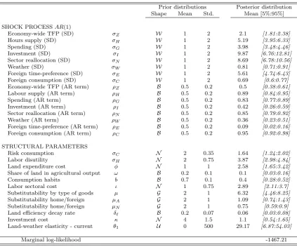
The rest of the parameters are estimated using Bayesian methods. Table 5 and Figure 6 report the prior (and posterior) distributions of the parameters for New Zealand. Overall, our prior distributions are either relatively diffuse or consistent with earlier contributions to Bayesian estimations such as Smets and Wouters (2007). In particular, priors for the persistence of the AR(1) processes, the labor disutility curvatureσH, the consumption habitsband the investment
adjustment cost κ are directly taken from Smets and Wouters (2007). The standard errors of the innovations are assumed to follow a Weibull distribution with a mean of 1 and a standard deviation of 2. The Weibull distribution is more diffuse than the Inverse Gamma distribution (both type 1 and 2), has a positive support and provides a better fit in terms of data density. Substitution parametersµ,µN, and µA are each assumed to follow a Gamma distribution with
a mean of 2 and a standard deviation of 1 in order to have a support that lies between 0 and 5. The risk aversion parameter σC is assumed to follow a Normal distribution with a mean of
2 and a standard deviation of 0.35 in the same vein as Smets and Wouters (2007). The labor sectoral costιfollows a diffuse Gaussian distribution with a mean of 1 and a standard deviation of 0.75, as the literature of two-sector models suggests that this parameter is above zero to get a positive correlation link across sectors. The land cost parameter φ is also assumed to follow a diffuse Gaussian distribution with prior mean and standard deviation both set to 1, so that the response of output is consistent with that of the VAR model.
Regarding priors for the agricultural sector, the land efficiency decay rate parameter δℓ is
assumed to follow a Beta distribution with prior mean and standard deviation of 0.2 and 0.1, respectively. This prior is rather uninformative as it allows this decay rate to be either close to 0 or close to 0.50, the latter would imply an annual decay rate of 200%. Regarding the land share in the production function ω, first, under decreasing return this parameter must be below 1, second, the economic literature suggests that this parameter is close to 20%.25 We thus impose a beta distribution with mean 0.2 and standard deviation 0.1. One of the key parameter in the paper is the damage function parameter θ and possibly subject to controversy. The literature on IAMs traditionally connects temperatures to output through a simple quadratic damage function in order to provide an estimation of future costs of carbon emissions on output. However,Pindyck(2017) raised important concerns about IAM-based outcome as modelers have so much freedom in choosing a functional form as well as the values of the parameters so that the model can be used to provide any result one desires. To avoid the legitimate criticisms inherent to IAMs, we adopt here a conservative approach on the value of this key parameter of
24The value of this parameter marginally affects the dynamic of the model, but it allows us to remove a unit
root component induced by the open economy setup.
25The share of landωin the production function is estimated at 15% for the Canadian economy byEchevarr´ıa
the damage function and set a very diffuse prior with a uniform distribution with zero mean and standard deviation 500.
4.3 Posterior Distribution
In addition to the prior distributions,Table 5reports the estimation results that summarize the means and the 5th and 95th percentiles of the posterior distributions, while the latter are illus-trated in Figure 6.26 According to Figure 6, the data were fairly informative, as their posterior distributions did not stay very close to their priors. However, we assess the identification of our parameters using methods developed by Iskrev (2010), these identification methods show that sufficient and necessary conditions for local identification are fulfilled by our estimated model.
1 2 3 0
0.5 1 1.5
σCcons. risk
0 2 4 6 8 0
0.2 0.4 0.6
σHlabor disutility
0 0.2 0.4 0
2 4 6 8
ωland share
0 0.2 0.4 0.6 0.8 0
2 4
bcons. habits
0 2 4 6 0
0.2 0.4 0.6 0.8
ιlabor sectoral cost
0 2 4 6 8 0
0.5 1
κinvestment cost
5 10 15 0
0.1 0.2 0.3 0.4
µsectoral subst.
2 4 6 0
1 2 3 4
µN non-farm subst.
0 2 4 6 0
0.5 1 1.5
µAfarm subst.
−2 0 2 4 6 0
0.2 0.4 0.6
φland expenditure cost
0 0.1 0.2 0.3 0.4 0
10 20
δℓland decay
−500 0 500 0
1 2 3
·10−2
θweather elasticity
[image:19.595.72.513.238.449.2]Prior Posterior
Figure 6: Prior and posterior distributions of structural parameters for New Zealand (excluding shocks).
While our estimates of the standard parameters are in line with the business cycle liter-ature (see, for instance, Smets and Wouters (2007) for the US economy or Lubik (2006) for New Zealand), several observations are worth making regarding the means of the posterior dis-tributions of structural parameters. Strikingly, the land-weather elasticity parameter θ has a high posterior value that is clearly different from 0. This implies that even with loose priors, the model suggests that variable weather conditions matter for generating business cycles con-sistently with empirical evidence of Kamber et al. (2013) and Mejia et al. (2018). The land expenditure costφsuggests that the returns to scale for land expenditures are quadratic. Sub-stitution seems to be an important pattern of consumption decisions of households, especially at a sectoral level. However, the substitution between home and foreign non-agricultural goods appears to be rather low, contrary to the substitution degree between agricultural and non agricultural goods that is remarkably high. Regarding the labor reallocation parameterιin the utility function of households, the data favor a costly labor reallocation across sectors, which is in line with the findings ofIacoviello and Neri(2010) for the housing market.
26The posterior distribution combines the likelihood function with prior information. To calculate the posterior
Model type M(θ= 0) M(θ6= 0)
Model description No Weather Damage Model Weather-Driven Business Cycles Damage function Ω εW
t
1 εW
t
−θ
Prior probability 1/2 1/2
Laplace approximation -1473.704 -1467.206
Posterior odds ratio 1.000000 663.6605
[image:20.595.68.513.71.161.2]Posterior model probability 0.001505 0.998495
Table 2: Prior and posterior model probabilities
To assess how well the estimated model captures the main features of the data, we report in Table 6andTable 7both the moments simulated by the model and their empirical counterpart. First, the model does a reasonably job through its steady state ratios in replicating the observed mean. The model performs quite well in terms of volatility for most of observable variables, except for total output and consumption as both are clearly overstated by the model while the theoretical volatility of foreign output is understated. The model performs very well at repli-cating the persistence of all observable variables. Finally regarding the correlation with GDP, the model replicates the sign of all the correlations, but not their full magnitude. In particular, the correlation with the foreign GDP is not captured by the model, this is a well known puzzle in international economic that can be easily solved by imposing a positive correlation across shocks in the model’s covariance matrix.
5
Do Weather Shocks Matter?
A natural question to ask is whether weather shocks significantly explain part of the business cycle. To provide an answer to this question, two versions of the model are estimated – using the same data and priors. In an alternative version of the model, which we consider as a benchmark, the damage function given in Equation 3is neutralized by imposing θ= 0. Under this assumption, any fluctuation in the weather has no implication for agriculture and thus does not generate any business cycles. In contrast, we compare the benchmark model with the version presented previously in the model section, characterized by the presence of weather-driven business cycles withθ6= 0.
Table 2reports for the two models the corresponding data density (Laplace approximation), posterior odds ratio and posteriors model probabilities, which allow us to determine the model that best fits the data from a statistical standpoint. Using a uninformative prior distribution over models (i.e., 50% prior probability for each model), we compute both posterior odds ratios and model probabilities taking the model M(θ= 0), i.e., the one with no weather damage as the benchmark.27 We conduct a formal comparison between models and refer toGeweke(1999) for a presentation of the method to perform the standard Bayesian model comparison employed inTable 2 for our two models. Briefly, one should favor a model whose data density, posterior odds ratios and model probability are the highest compared to other models.
We examine the hypothesis H0: θ = 0 against the hypothesis H1: θ 6= 0. To do this,
we evaluate the posterior odds ratio of M(θ6= 0) on M(θ= 0) using Laplace-approximated marginal data densities. The posterior odds of the null hypothesis of no significance of weather-driven fluctuations is 663.66:1 which leads us to strongly reject the null, i.e., weather shocks do matter in explaining the business cycles of New Zealand. This result is confirmed in terms of
27As underlined byRabanal (2007), it is important to stress that the marginal likelihood already takes into
log marginal likelihood and posterior odds ratio. This is an important result from the model that highlights the non-trivial role of the weather in driving the business cycles of New Zealand.
6
Weather Shocks as Drivers of Aggregate Fluctuations
This section discusses the propagation of a weather shock and its implications in terms of business cycle statistics.
6.1 Propagation of a Weather Shock
We first report the simulated Bayesian system’s responses of the main macroeconomic variables following a standard weather shock inFigure 7.28 We also report the responses from the VAR estimation for observable variables which are common between the VAR and the DSGE model. Unlike the VAR model, the DSGE model provides the underlying micro-founded mechanisms that drives the propagation of a weather shock.
From a business cycle perspective, this shock acts as a standard (sectoral) negative supply shock through a combination of rising hours worked and falling output. Consistently with the VAR model, a drought event strongly affects business cycles through a large decline in agricultural output (1.5%), as the weather influences land input in the production process of agricultural goods. Land productivity is strongly negatively affected by the drought. This result is in line with Kamber et al.(2013), as New Zealand’s farmers rely extensively on rainfall and pastures to support the agricultural sector. A drought shock decreases land productivity by 22% in the model. To compensate for this loss, farmers can use more non-agricultural goods as inputs to reestablish their land productivity. For instance, dairy or crop producers may require more water to irrigate their grasslands or cultures to offset the dryness. Farmers may also use more pesticides, as droughts are often followed by pest outbreaks (Gerard et al., 2013). The demand effect for these non-agriculture goods is captured in the model by a rise in inputsxitin
Equation 4, which results in an increase in land costs. The surge in non-agriculture goods has a positive side effect on non-agriculture output. Both the drop in the agricultural production and the rise in non-agriculture output alter the sectoral price structure. As the drought causes a reduction in the agricultural production and a rise in land costs, the relative price in the agricultural sector rises through a market cleaning effect. Since relative prices are negatively correlated, the price of non-agricultural goods declines in response, thus fueling the demand for non-agricultural goods. With respect to the VAR model, the DSGE model predicts a higher contraction of economic activity combined with a weaker response of the real exchange rate.
From an international standpoint, the decline in domestic agricultural production generates trade balance deficits. Two factors might explain this. First, around fifty percents of New Zealand’s merchandise exports are accounted for by agricultural commodities over the sample period. As both output and price competitiveness of the agricultural sector are deteriorated, New Zealand exports decline. However, the decline price in relative price of non-agricultural fuels the external demand for non-agricultural, thus explaining why this sector experiences a boom. Taken together, the effect of the agricultural sector outweighs the other sector, through a fall in the trade balance and the current account. In the meantime, the domestic real exchange rate depreciates driven by the depressed competitiveness of farmers, which helps in restoring their competitiveness. This reaction of the exchange rate is consistent with the prediction of the VAR model inFigure 4.
28The impulse response functions (IRFs) and their 90% highest posterior density intervals are obtained in a
6.2 The Contribution of Weather Shocks on Aggregate Fluctuations
Figure 8 reports the forecast error variance decomposition for four observable variablest, i.e., aggregate real production (gdpt), real agricultural production (YtA), real consumption (Ct) and
hours worked (Ht). Five different time horizons are considered, ranging from two quarters
(Q2), to ten (Q10) and fifty quarters (Q50) along with the unconditional forecast error variance decomposition (Q∞). In each case, the variance is decomposed into four main components related to supply shocks (technology, labor supply and sectoral reallocation shock), demand shocks (government spending, household preferences and investment shocks), foreign shocks (consumption and foreign preferences), and obviously the weather shocks.
For GDP (gdpt), supply shocks are the main drivers of the variance in both the short and
the long term, followed by demand and foreign shocks. Interestingly, we find that foreign shocks are a sizable driving force of output in the short run by contributing up to 18% of the volatility of GDP. UnlikeJustiniano and Preston(2010a) who find a trivial contribution of foreign shock in small open economy models, our model is able to capture the key role of foreign shock as a driver of economic fluctuations. Foreign shocks play a non-negligible role. They account for 27.6% of New Zealand’s production in the short run, and 11.8% in the long run. By increasing the time horizon, the contribution of supply, demand and foreign shocks tends to reduce and are gradually replaced by weather shocks, starting from 2% at two-quarter horizon to 30% for the unconditional variance.
Turning to agricultural production, supply shocks account for most fluctuations in the short run. They are responsible for 85% of the variance of agricultural production at one-quarter horizon. Domestic and foreign demand shocks play a trivial role in the volatility of agricultural production. The importance of supply shocks declines in the long run, although remaining non-negligible, explaining 58% of agricultural production for the unconditional variance. Weather shocks remarkably drive the variance of agricultural production after a time lag of two quarters. In addition, increasing the time horizon magnifies this result. Thus the weather is a key deter-mining factor of agricultural fluctuations according to the theoretical representation of the data by our model. Concerning the variance of consumption, it is mainly affected, in the short term, by foreign shocks. Weather shocks play a significant role in the same way as for agricultural production, starting from a more distant time horizon. Finally for working hours, they are only slightly affected by weather shocks. Supply shocks are the main drivers of the variance of hours worked as they drive most of the variance of hours.
Overall, we find that weather shocks cause important macroeconomic fluctuations. The increasing contribution of the weather in the time horizon highlights an interesting persistence mechanism which can be associated to the weather hysteresis effects discussed in the business cycle evidence section.
6.3 Historical Decomposition of Business Cycles
An important question one can ask of the estimated model is how important were weather shocks in shaping the recent New Zealand macroeconomic experience. Figure 9 displays the year-over-year growth rate in per capital of real agricultural production, GDP, consumption and hours worked. The blue dotted line is the result of simulating our model’s response to all of the estimated shocks and to the initial conditions. The dotted line shows the result of this same simulation when we feed our model only the weather shock.