Munich Personal RePEc Archive
Structural changes in exchange
rate-stock returns dynamics in South
Africa: Examining the role of crisis and
new trading platform
Phiri, Andrew
10 April 2018
Online at
https://mpra.ub.uni-muenchen.de/85826/
STRUCTURAL CHANGES IN EXCHANGE RATE-STOCK RETURNS DYNAMICS IN SOUTH AFRICA: EXAMINING THE ROLE OF CRISIS AND NEW
TRADING PLATFORM
A. Phiri
Department of Economics, Faculty of Business and Economic Studies, Nelson Mandela
Metropolitan University, Port Elizabeth, South Africa, 6031.
ABSTRACT: The 2007 sub-prime crisis and the adoption of Millennium trading platform
represent two of the most important recent structural developments for the Johannesburg
Stock Exchange (JSE). Under an environment of flexible and volatile exchange rates, this
study seeks to examine the effects of these two structural events on the exchange rate-equity
returns nexus for 4 JSE indices using the nonlinear autoregressive distributive lag (N-ARDL)
cointegration. We use monthly data collected from 2000:M01 to 2017:M12, and conduct our
empirical analysis over sub-periods corresponding to breaks caused by the crisis and the use
of a new trading platform. We find prior the crisis exchange rates appreciations generally
cause stock returns whereas depreciations are unlikely to cause stock returns to decrease.
However, during crisis period this relationship entire disappears whilst resurfacing
subsequent to the adoption of a new trading platform although the dynamics of the time series
differs between sectors. Our overall empirical results caution regulatory authorities to closely
monitor stock market developments as the new trading platform offers market participants
opportunities of using the exchange rate to beat the market.
Keywords: Stock returns; Exchange rates; High frequency trading; Millennium trading
platform; N-ARDL model; Flexible Fourier form unit root test; South Africa; Emerging
economies.
1 INTRODUCTION
The world has experienced increasing global financial integration over the last couple
of decades or so, mainly in the form of financial liberalization and improved international
capital flow movements. This became exceedingly apparent following the infamous crash of
the US financial system triggered by the sub-prime mortgage crisis of 2008, which had
contagion spill-over effects to financial markets worldwide. The most immediate
international effects of the sub-prime crisis were exerted on the dollar exchange rate with
other international currencies as well as on stock markets globally. It is for this reason that
many economists have recently taken a keen interest on the empirical relationship between
the exchange rate and stock market returns (Bahmani-Oskooe and Saha (2015, 2016, 2018)).
Even though it is widely acknowledged that the adverse effects of the global financial
crisis has varied across financial markets worldwide, the general consensus is that African
financial systems responded more resiliently towards the aftereffects of the crisis. Notably,
many African economies are characterized by underdeveloped stock markets and monetary
authorities in a number of these countries have attempted to keep currency exchanges
competitive by relying on floating exchange rate policies as guided by the “Washington consensus”. Thus far, the contagion effects arising from the financial crisis have not severely
altered stock market dynamics in less developed African stock exchanges seeing that many of
these stock markets are not well integrated with other international financial and capital
markets. However, many African currencies have turned out to be quite volatile against the
US dollar following the 2007 sub-prime crisis and the more recent oil price hikes of
2012-2014 and this, by itself, poses as a major threat to financial as well as economic stability in
these economies.
In retrospective, the South African economy presents a unique case for the African
continent as her financial system is characterized by a blend of a mature stock market and a
highly institutionalized ‘full-fledged’ inflation targeting regime monetary policy framework.
equity markets on the continent, with the Johannesburg Stock Exchange (JSE) boasting the
highest market capitalization in Africa, with the highest number of cross-listed firms on the
continent and being the only country to have incorporated high frequency trading (HFT)
trading mechanism into trading platforms in 2013 (Phiri, 2016). This later feature not only
represents a technological advantage over other African economies but more importantly
represents a structural change in trading dynamics with respect to the major improvement in
speed and volumes of transactions. Moreover, the country has one of the strongest currencies
in the Sub-Saharan African (SSA) region and lists the highest amount of foreign reserves
which more-or-less reflects the confidence or preference which foreign entities have in
exchanging their domestic currency for South African Rands.
Against these attributes, it is therefore not at all surprising that there have been a
handful of previous studies which have examined the relationship between the Rand/Dollar
(ZAR/US$) exchange rate and JSE equity returns (Ocran (2010), Adjasi et. al. (2011), Alam
et al. (2011), Ndako (2013), Mlambo et al. (2013), Sui and Sun (2015) and Fowowe (2015)).
Nonetheless, these studies suffer a number of shortcomings. Firstly, a majority of those
studies tend to rely on linear cointegration frameworks such as such as those presented by
Engle-Granger (1987), Johansen (1991) and Pesaran et al. (2001). However, as argued by
Bahmani-Oskooee and Saha (2015, 2018), given that market participants in stock markets
base their decisions on expectations, then most likely exchange rates would have a nonlinear
influence on stock prices. Secondly, a number of these studies employ time series
corresponding to periods prior to the financial crisis hence ignore the possibility of changing
dynamics of the exchange rate-stock returns dynamics caused by the crisis (Ocran (2010),
Adjasi et al. (2011) and Alam et al. (2011)). Thirdly, even when studies employ data covering
the financial crisis period, the authors fail to adequately account for this structural break
primarily due to reliance on linear cointegration models (Ndako (2013), Mlambo et al.
(2013), Sui and Sun (2015) and Fowowe (2015)). Fourthly, previous studies have not
considered the possibility of a second structural break brought about by the adoption of the
Millennium trading platform which has ushered in the ‘much-celebrated’ high frequency
aggregated stock indices which heightens the possibility of aggregation bias associated with
these previous studies.
In our study we apply the recently introduced nonlinear autoregressive distributive lag
(N-ARDL) model of Shin et al. (2014) to examine nonlinear cointegration between the
Rand-Dollar exchange rate and the returns on four JSE stock indices; namely the i) the All-Share
index ii) the Top.40 index iii) the financial 25 index and iv) the Resource.10 index. The
N-ARDL models main appealing feature is that in similarity to its linear predecessor, the N-ARDL
model of Pesaran et al. (2001), this framework permits the modelling of long-run and
short-run asymmetric cointegration effects between a combination of levels and first difference
stationary variables. Notably, this model framework has been successfully used to model
short-run and long-run asymmetric cointegration relationships between stock returns and
exchange rates for the industrialized and other emerging economies (Cuestas and Tong
(2015), Bahmani-Oskooee and Saha (2015, 2017, 2018) and Tong (2018)) but is yet to be
applied to African time series. We therefore contribute to this emerging group of literature by
employing the N-ARDL framework to South African monthly time series covering the post
Asian financial crisis period of 2000:M01 to 2017:M12 and further account for the 2007
financial crisis and the adoption of the new Millennium trading platform in our analysis.
Having provided a background, the remainder of the study is structured as follows.
The next section provides a review of the related literature. The third section of the paper
presents the empirical data and unit root tests of the time series. The fourth section reports the
empirical estimates of the empirical models whereas the paper is concluded in the fifth
section of the paper in the form of policy recommendations and avenues for future research.
2 LITERATURE REVIEW
Empirical interest concerning the relationship between exchange rates and stock
prices gained significant prominence following the demise of the Bretton Woods system and
worldwide in the mid-1970’s. Further exacerbating the need for such research in the 1980’s, were the formation of the Plaza accord agreement of 1985 and the Louvre Accord agreement
of 1987 which aimed to stabilize the international currency market via a devaluation of the
dollar against the currencies of G5 economies. It therefore comes as no surprise that a bulk
majority of earlier empirical studies which examined the exchange rate-stock price
relationship where typically focused on the US economy with the works of Dornbusch and
Fischer (1980), Branson (1983), Frankel (1983) and Gavin (1989) being classic theoretical
contributions. On one hand, Dornbusch and Fischer (1980) and Gavin (1989), develop the
flow-oriented or the goods-market approach to exchange rate determination which assumes
that changes in the exchange rates affect international competitiveness and the trade balance,
which in turn affects the real output and firm’s performance, which is ultimately reflected in
stock prices. On the other hand, Branson (1983) and Frankel (1983) propose the
stock-oriented model or portfolio-balance approach which specifically shows that exchange rates
are affected by stock price movements via the capital account since stock market movements
lead to money flow into or out of the countries, which affects the demand for money, and
thereby leading to changes in interest rates as well as exchange rate movements.
Accompanying these theoretical underpinnings were the earlier prominent empirical
contributions of Franck and Young (1972), Aggarwal (1981), Solnik (1987) and Ma and Kao
(1990). Nevertheless, the inferences drawn from these earlier studies were branded as
unreliable based on the premise of these studies ignoring I(1) stochastic trends in the time
series variables and thus providing the possibility of the regression estimates being spurious.
Henceforth emerged a separate group of earlier empirical works which began to utilize
cointegration techniques, most notably the two-stage cointegration procedure of Engle and
Granger (1987) and Johansen’s (1991) vector error correction model (VECM), in their empirical analysis which set a trend for research output on the subject matter during the
1990’s with a primary focus on industrialized economies (Bahmani-Oskooe and Sohrabian
(1992), Smith (1992) and Mok (1993), Ajayi and Mougoue (1996), Ajayi et al. (1998) and
The Asian contagion crisis in 1998-1999 sparked a flurry of research interest
concerned with examining the exchange rate-stock return nexus with specific reference to
Asian economies. Prominent examples amongst this group of studies include the individual
country analysis of Mishra (2004) and Ramasamy and Yeung (2005) for India; Zhao (2010)
and Rutledge et al. (2014) for China as well as the panel group studies of Abdalla and
Murinde (1997) for India, Korea, Pakistan and Philippines; Granger et al. (2000) for Hong
Kong, Indonesia, Japan, South Korea, Malaysia, the Philippines, Singapore, Thailand and
Taiwan; Smyth and Nanda (2003) for Bangladesh, India, Pakistan and Sri Lanka; Phylaktis
and Ravazzolo (2005) for Hong Kong, Malaysia, Singapore, Thailand and Philippines; Yau
and Nieh (2006) for Taiwan and Japan; Liu et al. (2007) for Malaysia, Singapore, Korea,
Philippines, Japan, Germany and the UK; Pan et al. (2007) for Hong Kong, Japan, Korea,
Malaysia, Singapore, Taiwan, Thailand; Lean et al. (2011) for Hong Kong, Indonesia, Japan,
Korea, Malaysia, the Philippines, Singapore and Thailand; Lin (2012) for India, Indonesia,
Korea, Philippines, Thailand and Taiwan; as well as Liang et al. (2013, 2015) for Indonesia,
Malaysia, Philippines, Singapore and Thailand. Regardless of the extensive nature of these
studies, the empirical evidence acquired from this cluster of studies, so far, can be best
described as being inconclusive.
The world experienced yet another catastrophic financial crisis in September 2009,
when the Lehman Brothers filed for the Chapter 11 bankruptcy protection thus leading to the
US national banking crisis which propagated to global financial markets. It was following the
advent of this sub-prime crisis that a majority of the empirical literature conducted for the
South African economy emerged, with the study of Ocran (2010) being the earliest study to
examine the exchange rate-stock price relationship for the economy. Following Ocran’s (2010) study, other empirical works on the exchange rate-stock returns relationship for the
South African economy began to emerge and the most prominent studies existing up-to-date
include the country-specific studies of Alam et al. (2011), Mlambo et al. (2013) as well as the
panel based works of Adjasi et al. (2011), Ndako (2013), Sui and Sun (2015), Fowowe
(2015) and Dahir et al. (2017). Notably a majority of these previous South African studies
(2013), Mlambo et al. (2013) and Sui and Sun (2015)) or in instances where cointegration is
found, there were no causality effects (Ocran (2010), Alam et al. (2011) and Fowowe et al.
(2015)).
It was also subsequent to the global financial crisis that research on the subject matter
began to take a new empirical direction with economists contemplating on a possible
nonlinear relationship between exchange rates and stock prices. The rationale behind this
school of thought is that the relationship between exchange rates and stock prices is
non-monotonic and exchange rate exposure is different for periods of currency as compared to
currency depreciation. Nonlinear studies existing in the literature up-to-date include the
works of Tabak (2006) for Brazil; Kumar (2009) for India; Yau and Nieh (2009) for Japan
and Taiwan; Tsai (2012) for Singapore, Thailand, Malaysia, Philippines, South Korea and
Taiwan; Cakan and Ejra (2013) Turkey, Thailand, Brazil, India, Korea, Mexico, Philippines,
Poland, Russia, Singapore and Taiwan; Chkili and Nguyen (2014) for Brazil, Russia, India,
Chana and South Africa; Dar et al. (2014) for India, Pakistan, Bangladesh, Sri Lanka,
Malaysia, Indonesia, Philippines and Thailand; Ali et. al. (2015) for South Africa;
Koulakiotis et al (2015) for the US, Canada and UK; Ho and Huang (2015) for Brazil,
Russia, India and China; Bahamani-Oskooee and Saha (2015) for the US; Bahamani-Oskooee
and Saha (2016) for Brazil, Canada, Chile, Indonesia, Japan, Korea, Malaysia, Mexico and
the UK; Cuestas and Tang (2017) for 31 Chinese industries; Bahamani-Oskooee and Saha
(2017) for Argentina, Australia, Austria, Belgium, Brazil, Canada, Chile, China, France,
Germany, Greece, Hong Kong, India, Indonesia, Japan, Korea, Malaysia, Mexico,
Netherlands, New Zealand, Singapore, Switzerland, UK, US; and Tang (2018) for 87 Chinese
auto firms.
Initially, a majority of these ‘nonlinear’ studies relied on MTAR cointegration
framework (Yau and Nieh (2009), Ali et al. (2015), and Koulakiotis et al. (2015)), nonlinear
causality tests (Tabak (2006), Kumar (2009), Cakan and Ejra (2013) and Ho and Huang
(2015)) as well as quantile regressions (Tsai (2012) and Dar et al. (2014)). However, recent
modelling both short-run and long-run cointegration asymmetries between time series with
different integration properties (i.e. Bahmani-Oskooee and Saha (2016, 2017), Cuestas and
Tang (2017) and Tang (2018)). Even though these ‘nonlinear studies’ collectively produce different results for different economies, what is encouraging is that they commonly
advocated for the exchange rate-stock price nexus as being asymmetric over the steady-state.
For the sake of brevity and convenience the findings of these nonlinear studies along with the
others reviewed in this section are summarized in Appendix A.
3 EMPIRICAL FRAMEWORK
The traditional analytical framework testing the link between stock markets and
exchange rates is based on the influence of the exchange rate on firm profitability and share
prices firms as modelled by Jorion (1990) and further expounded in the study of Bodnar and
Gentry (1993). According to this framework, stock market returns (smrt) is modelled as being
endogenous to exchange rate (ext):
𝑠𝑚𝑟𝑡 = 0+ 1𝑒𝑥𝑡+ 𝑡 (1)
Where µt is a well-behaved error term with a zero mean and constant variance. As
previously mentioned earlier studies focused on estimating equation (1) using linear
cointegration models. However, nonlinear models as introduced, as firstly introduced in the
seminar work of Balke and Fomby (1997) have emerged as a more appealing alternative.
Nonetheless, many of the existing nonlinear cointegration models (i.e. Enders and Granger
(1998), Enders and Siklos (2001), Lo and Zivot (2001) and Hansen and Seo (2002)) are too
restrictive in the sense of requiring the time series to be integrated of similar order and
typically focuses on short-run equilibrium asymmetries whilst ignoring crucial long-run
asymmetries. Henceforth, the N-ARDL model of Shin et al. (2014) has been recently relied
on in the literature to model short-run and long-run asymmetries between exchange rates and
processes of positive and negative changes (i.e. SRt = EX0 + 𝐸𝑋𝑡++ 𝐸𝑋𝑡−), such that equation
(1) can be re-specified as the following long-run asymmetric model:
SRt = 0+ β+𝐸𝑋𝑡++ β-𝐸𝑋𝑡− + et (2)
Where 𝑆𝑅𝑡+ = 𝑖𝑗=1 𝑆𝑅𝑗+ = 𝑖𝑗=1max(SRj, 0) and 𝐸𝑋𝑡− = 𝑖𝑗=1 𝐸𝑋𝑗− =
min
𝑖
𝑗=1 (EXj, 0). The NARDL (p, q)-in-levels transformation of regression (4) can be
given as:
𝑆𝑅𝑡= 𝑗𝑝=1𝜓𝑖𝑆𝑅𝑡−𝑗+ 𝑝𝑗=1 𝑗+𝐸𝑋𝑡+−𝑗+ 𝑗−𝐸𝑋𝑡−−𝑗 + 𝑡 (3)
Whereas the associated error correction representation can be denoted as:
𝑆𝑅𝑡= 𝑗𝑝=1 𝑖𝑆𝑅𝑡−𝑗+ 𝑗+𝐸𝑋𝑡+−𝑗+ 𝑗−𝐸𝑋𝑡−−𝑗+ 𝑝𝑗=1−1 𝑖 𝑆𝑅𝑡−𝑗+ 𝑞𝑗=0−1( 𝑗+ 𝐸𝑋𝑡+−𝑗+
𝑗− 𝐸𝑋𝑡−−𝑗) + 𝑡 (4)
The asymmetric long-run parameters of interest from equations (3) and (4) are
thereafter computed as β+
= -(+/) and β- = -(-/). To validate the NARDL long-run and short-run effects, Shin et al. (2014) propose the testing of three empirical hypothesis. The
first, is an asymmetric extension of the conventional bounds test for cointegration (Pesaran et
al., 2001) and tests the null hypothesis of = + = -. The second hypothesis tests the null of
no long-run cointegration effects (i.e. β-= β+) whilst the third tests the null hypothesis of no
short-run asymmetric effects (i.e. 𝑞𝑖=0−1 𝑗+ = 𝑞𝑖=0−1 𝑗−).
4 DATA AND EMPIRICAL RESULTS
The empirical data used in our study is collected from the INET BFA online database
and consists of five time series variables, namely, the closing values of i) the Rand-Dollar
exchange rate, ii) the FTSE/JSE All Share index, iii) the FTSE/JSE Top.40 index, iv) the
FTSE/JSE Industrial 25 index and v) the FTSE/JSE Resource.10 index. All utilized time
series are collected over monthly frequencies for the period of January 2000 to December
2017 and we have chosen this sample period because it strictly reflects developments in the
JSE which have occurred subsequent to the outfall of open outcry platforms and
incorporation of fully automated trading systems. Our sampled data further coincides with an
era of flexible exchange rate regime in which currency is determined by market forces
without direct intervention by the Reserve Bank.
By design our dataset begins during a period when the London Stock Exchange Stock
Exchange Electronic Trading System (i.e. LSE-SETS) was officially adopted as the JSE’s main trading platform in 2001, just subsequent to the Asian financial crisis and Dot.com
bubble burst of 1999 and 2000, respectively. In 2007, just around the advent of the filing of
Chapter 11 bankruptcy by the Lehman Brother, the LSE leased yet another trading platform
to the JSE i.e. JSE trade elect system, and in 2013, the JSE shifted its trading platform from
London to Johannesburg under the banner of the Millennium exchange. Note that it is under
this trading platform that high frequency trading was ushered into the JSE hence allowing for
the speed of transactions to be executed at approximately 400 times faster than under the
previous trading platforms (Phiri, 2017). Further note that our study covers all these
important structural events which need to be accounted for in our empirical analysis. For
empirical purposes, we transform the raw stock prices time series data into returns using the
following continuous compounded returns formulae:
R = log (pt) - log (pt-1) (5)
Where R is the compounded returns, pt is the price index and pt-1 is the price index in
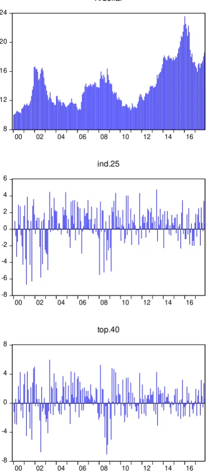
the previous period. The time series plots of the equity returns are provided in Figure 1 whilst
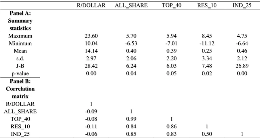
25 has the highest average returns (0.46%), followed by the all-share (0.40%), top 40 (0.39%)
and lastly resource 10 (0.25%). Conversely, resources 10 has the highest volatility (3.34),
followed by top 40 (2.20), industrials 25 (2.12) and all-share (2.06). The Rand/Dollar
exchange rate has generally been rising (deteriorating) from the beginning to the end of our
sample period with a minimum of 10.04 ZAR/US$ in 2001:M01 to an all-time high of 23.60
ZAR/US$ in 2016:M01. The preliminary correlation estimates indicate that exchange rates
are negatively correlated with the JSE equity returns, that is, an exchange rate appreciation
(depreciation) strengthens (weakens) JSE equity returns, even though these correlations are
difficult to visually ascertain from the time series plots in Figure 1. This last point may be due
[image:12.595.66.525.349.590.2]to the observed weak correlations identified between the exchange rate and JSE returns.
Table 2: Summary statistics and unit root tests
R/DOLLAR ALL_SHARE TOP_40 RES_10 IND_25
Panel A: Summary
statistics
Maximum 23.60 5.70 5.94 8.45 4.75 Minimum 10.04 -6.53 -7.01 -11.12 -6.64
Mean 14.14 0.40 0.39 0.25 0.46 s.d. 2.97 2.06 2.20 3.34 2.12 J-B 28.42 6.24 6.03 7.48 26.89 p-value 0.00 0.04 0.05 0.02 0.00
Panel B: Correlation
matrix
R/DOLLAR 1
ALL_SHARE -0.09 1
TOP_40 -0.08 0.99 1
RES_10 -0.11 0.84 0.86 1
IND_25 -0.06 0.85 0.83 0.50 1
Nevertheless, a number of interesting visual observations can be deduced from the
individual series plots in Figure 1. For instance, the ZAR/US$ exchange rate has been mainly
affected by global distortions such as the oil price spikes of 2002-2003, the Lehman
bankruptcy of 2007 as well as the second oil spikes of 2012-2014. Similarly, all JSE returns
series have been influenced by the oil price hikes of 2002-2003 as well as by the global
financial crisis of 2007, although recovery from these exogenous shocks is evidently
adoption of HFT mechanism in 2013, the series have been less volatile and, with exception of
resources, the remaining series have been barely influenced by the advent of the second oil
price hikes of 2012-2014. Lastly we note that for all observed time series the Jarque-Bera
(J-B) statistic concludes on non-normality of the variables, as is expected from the financial
[image:13.595.73.284.241.720.2]time series and further advocates for existing asymmetries in the time series.
Figure 1: Time series plots of variables
8 12 16 20 24
00 02 04 06 08 10 12 14 16
R/dollar
-8 -6 -4 -2 0 2 4 6
00 02 04 06 08 10 12 14 16
all.share
-8 -6 -4 -2 0 2 4 6
00 02 04 06 08 10 12 14 16
ind.25
-15 -10 -5 0 5 10
00 02 04 06 08 10 12 14 16
res.10
-8 -4 0 4 8
00 02 04 06 08 10 12 14 16
top.40
Even though the N-ARDL model does not require formal testing of unit roots within
the variables, we consider it important to test the integration properties of the employed time
series since the integration properties may reveal important information concerning the
efficiency of the JSE. In particular, the weak-form efficient market hypothesis (EMH)
insinuates that the stationarity of stock returns series reflects an efficient capital market in the
sense that investors cannot obtain abnormal returns based on the historic security information
as anticipated events are already integrated into the present stock price (Phiri, 2015).
However, conventional unit root tests such as the ADF, PP, KPSS and DF-GLS tests ignore
nonlinearity and further fail to account for important structural breaks existing within the
data. Therefore, in following Kapetanois et al. (2003), we specify the following modified
Dickey-Fuller unit root testing regression:
Yt = ψi𝑌𝑡3−𝑖 + 𝑗𝑝=1 𝑖 𝑌𝑡−𝑖 + et (6)
Where the is a first difference operator of time series Yt, and the unit root null
hypothesis is tested as H0: ψi = 0 using the test statistic (DFKSS) computed as:
tADF = 𝑆.𝐸𝜓.(𝜓 ) (7)
With S.E.(𝜓) is the standard error of the coefficient estimate 𝜓. In order to account
for structural breaks we augment the KSS regression with a flexible Fourier function (FFF)
resulting the following test regression:
Yt = i𝑌𝑡3−𝑖 + 𝑝𝑗=1 𝑖 𝑌𝑡−𝑖+𝑎𝑖sin 2𝜋𝐾𝑡𝑇 +𝑏𝑖𝑐𝑜𝑠(2𝜋𝐾𝑡𝑇 ) + et, t = 1,2,…,T. (8)
Where K is the singular approximated frequency selected for the approximation,
unit root null hypothesis is thus tested as H0: i = 0 which is evaluated using the following
test statistic:
tKSS-FF = 𝑆.𝐸.( ) (9)
Enders and Lee (2012) place emphasis on estimating a Fourier function with a
singular frequency to avoid problems of over-fitting and loss of regression power. Moreover,
Enders and Lee (2012) propose that regression (12) be estimated for all integer values of K
which lie between the interval [1, 5] and selecting the estimation which produces the lowest
sum of squared residuals (SSR). The empirical results from these testing procedures is
summarized in Table 3 with Panel A reporting the results for the KSS test performed without
[image:15.595.66.532.409.579.2]a FFF function whilst Panel B reports the results for the test performed with a FFF function.
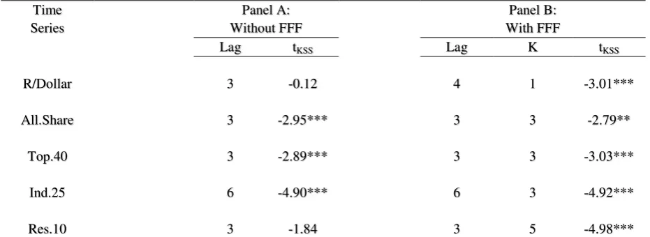
Table 3: KSS unit root test results with and without the FFF
Time Series
Panel A: Without FFF
Panel B: With FFF
Lag tKSS Lag K tKSS
R/Dollar 3 -0.12 4 1 -3.01***
All.Share 3 -2.95*** 3 3 -2.79**
Top.40 3 -2.89*** 3 3 -3.03***
Ind.25 6 -4.90*** 6 3 -4.92***
Res.10 3 -1.84 3 5 -4.98***
Note: “***”, “**”, “*” represent the 1%, 5% and 10% significance levels, respectively. The critical values associated with KSS tests are
-2.82 (1%), -2.22(5%) and -1.92 (10%).
Judging from the empirical results reported in Table 3, we note that when the KSS
unit root test is performed without a flexible Fourier function there exists evidence of a unit
root in both the ZAR/USD series and the Resource 10 returns, whilst the remaining time
series reject the unit root null hypothesis at all significance levels. However, when the FFF is
include in the KSS testing procedure all observed time series unanimously indicate the
and the Resource 10 time series rejecting the null hypothesis at all critical levels whereas the
All.Share returns reject the unit root null at a 5 percent critical level. Collectively, these
results provide strong evidence that once nonlinearity and structural breaks are accounted for
then the JSE is generally an efficient stock market.
4.3 Exchange rate and stock returns around the global financial crisis
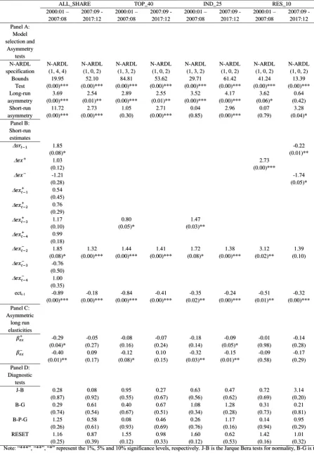
Table 4 presents the empirical findings of the pre and post crisis eras for the
All-Share, Top.40, industrial 25 and resources 10 indices. The order of our reportings
systematically corresponds to the modelling procedure used in obtaining our empirical
results. For instance, Panel A of Table 4 initially presents the lag selection results for all 8
N-ARDL models using the minimal values of the AIC and SC as information criterion in
determining the optimal lag for regressions. And then in the same panel, the three asymmetric
cointegration tests for i) nonlinear ARDL effects ii) long-run asymmetric effects iii) short-run
asymmetric effects are thereafter reported. As can be witnessed, all three forms of
asymmetries are unanimously verified for all estimated regression with the sole exception of
short-run asymmetric effects for the Top.40 returns in the pre-crisis period; the industrial 25
returns in the pre-crisis period; and both sub-periods for the Resource.10 returns.
Thereafter, Panel B presents the short-run and error correction estimates whilst the
long-run estimates are reported in Panel C reports the long-run regression coefficients and for
convenience sake only the normalized long-run elasticities are reported. Starting with the
short-run results in Panel B, we find that a majority of the estimated short-run coefficients are
positive and statistically significant at critical levels of at least 10 percent with the exception
of the short-run coefficients associated with the resource sector in the post-crisis periods
where the coefficients turn negative and significant. This implies that over the short-run an
increase in the ZAR/USD rate (i.e. depreciation of the Rand to the Dollar) is associated with
an increase in stock returns and vice versa, with the exception of the resource sector in the
post-crisis period. These findings are reminiscent of the flow-oriented hypothesis of Branson
significant error correction terms further indicate that disequilibriums in the dynamic system
are corrected over the steady-state for all equity returns. Against these findings it is
imperative to determine whether these short-run dynamics translate into significant long-run
effects.
Concerning the long-run coefficients reported in Panel C, we notice a switch in the
sign of regression coefficients from being dominantly negative and statistically significant in
the pre-crisis to being generally statistically insignificant in the post-crisis with the exception
of Industrials returns. In particularly, we observe that for the pre-crisis, a percentage
depreciation in the ZAR/USD rate results in a 0.29 decrease in All-Share returns whereas a
percentage appreciation in the ZAR/USD rate causes a 0.40 increase in All-Share returns.
Similar dynamics are observed in the post-crisis for the Industrials.25 returns, in which a
percentage appreciation in the exchange rate results in a 0.09 percentage decrease in returns
whilst a percentage depreciation in exchange rate reduces returns by 0.15 percent. Notably,
these nonlinear dynamics are in accordance with those found for other emerging economies
as in Tang (2018) for B-share firms in China (Tang (2018)) as well as in Bahmani-Oskooee
and Saha (2018) for Argentina and Malaysia.
Concerning the Top 40 returns and Industrials 25 returns in the pre-crisis an
appreciation of the exchange by one percentage point reduces stock returns by -0.12 percent
for Top.40 and -0.32 percent for Industrials whereas an appreciation of currency has no effect
on these stock returns. These dynamics replicate those of Bahmani-Oskooee and Saha (2016)
for the US and Malaysia as well as Bahmani-Oskooee and Saha (2018) for Mexico. On the
other hand, we observe neither appreciations of depreciation of currency has any significant
effects on stock returns in the post-crisis period for the all-share, top.40 and resource returns
and this is coherent with the findings of Bahmani-Oskooee and Saha (2018) for the US and
Table 4: Exchange rate-stock returns relationship for the pre- and post- crisis era
ALL_SHARE TOP_40 IND_25 RES_10 2000:01 –
2007:08
2007:09 - 2017:12
2000:01 – 2007:08
2007:09 - 2017:12
2000:01 – 2007:08
2007:09 - 2017:12
2000:01 – 2007:08 2007:09 - 2017:12 Panel A: Model selection and Asymmetry tests N-ARDL specification N-ARDL (1, 4, 4)
N-ARDL (1, 0, 2)
N-ARDL (1, 3, 2)
N-ARDL (1, 0, 2)
N-ARDL (1, 3, 2)
N-ARDL (1, 0, 2)
N-ARDL (1, 0, 2)
N-ARDL (1, 0, 2) Bounds Test 19.95 (0.00)*** 52.10 (0.00)*** 84.81 (0.00)*** 53.62 (0.00)*** 29.71 (0.00)*** 61.42 (0.00)*** 41.24 (0.00)*** 13.39 (0.00)*** Long-run asymmetry 3.69 (0.00)*** 2.54 (0.01)** 2.89 (0.00)*** 2.55 (0.01)** 3.52 (0.00)*** 4.17 (0.00)*** 3.62 (0.06)* 0.64 (0.42) Short-run asymmetry 11.72 (0.00)*** 2.73 (0.00)*** 1.05 (0.30) 2.71 (0.00)*** 0.04 (0.85) 2.96 (0.00)*** 0.07 (0.79) 3.28 (0.04)* Panel B: Short-run estimates
𝑠𝑟𝑡−1 1.85
(0.08)*
-0.22 (0.01)**
𝑒𝑥+ 1.03
(0.12)
2.73 (0.00)***
𝑒𝑥− -1.21
(0.28)
-1.74 (0.05)*
𝑒𝑥𝑡+−1 0.54
(0.45)
𝑒𝑥𝑡+−2 0.76
(0.29)
𝑒𝑥𝑡+−3 1.17
(0.10)
0.80 (0.05)*
1.47 (0.03)**
𝑒𝑥𝑡+−4 0.99
(0.18)
𝑒𝑥𝑡−−2 1.85
(0.08)* 1.32 (0.00)*** 1.44 (0.00)*** 1.41 (0.00)*** 1.72 (0.08)* 1.38 (0.00)*** 3.12 (0.02)** 1.39 (0.10)
𝑒𝑥𝑡−−3 -0.76
(0.50)
𝑒𝑥𝑡−−4 1.00
(0.35) ectt-1 -0.89
(0.00)*** -0.18 (0.00)*** -0.84 (0.00)*** -0.41 (0.00)*** -0.35 (0.02)** -0.24 (0.00)*** -0.51 (0.01)** -0.32 (0.00)*** Panel C: Asymmetric long run elasticities
𝛽𝑒𝑥+ -0.29
(0.04)* -0.05 (0.27) -0.08 (0.16) -0.07 (0.24) -0.18 (0.14) -0.09 (0.05)* -0.01 (0.98) -0.14 (0.28)
𝛽𝑒𝑥− -0.40
(0.01)** 0.09 (0.17) -0.12 (0.08)* 0.10 (0.15) -0.32 (0.03)** -0.15 (0.01)** -0.09 (0.58) -0.17 (0.29) Panel D: Diagnostic tests
J-B 0.28 (0.87) 0.08 (0.92) 0.95 (0.55) 0.27 (0.67) 0.63 (0.56) 0.47 (0.62) 0.72 (0.69) 3.14 (0.20) B-G 0.29
(0.74) 0.61 (0.54) 0.40 (0.67) 0.67 (0.51) 1.08 (0.34) 1.28 (0.28) 0.31 (0.73) 0.21 (0.81) B-P-G 1.25
(0.26) 0.58 (0.61) 0.08 (0.93) 0.46 (0.69) 0.26 (0.76) 1.17 (0.16) 0.14 (0.94) 0.95 (0.29) RESET 1.16
(0.25) 0.87 (0.39) 1.55 (0.12) 0.98 (0.33) 1.60 (0.12) 0.62 (0.53) 1.42 (0.16) 1.01 (0.32)
Note: “***”, “**”, “*” represent the 1%, 5% and 10% significance levels, respectively. J-B is the Jarque Bera tests for normality, B-G is the
function form and indicate that errors from all estimate regressions are normal, homoscedastic are free from autocorrelation as well as the regressions being of correct function form.
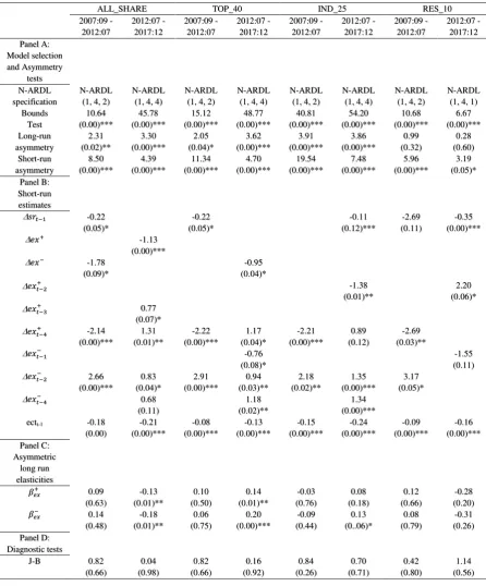
4.4 Exchange rate and stock returns around the adoption of a new trading platform
Having validated the proposition that the exchange rate-stock returns relationship has
changed from being generally significant in the pre-crisis period to being absent in the
post-crisis period, we now examine whether the adoption of the Millennium trading platform has
altered this relationship in the post-crisis periods. To this end, we provide the N-ARDL
estimates corresponding to the pre- Millennium periods and post- Millennium periods for all
equity returns which are reported in Table 5. Once again Panel A reports the selected
N-ARDL specifications based on the AIC and SC information criterion which are accompanied
by their respective tests for asymmetric ARDL effects, long-run asymmetries and short-run
asymmetries. The findings indicate that all regressions reject the three null hypotheses of no
N-ARDL effects, no-long-run asymmetries and no short-run asymmetries for all stock returns
in both sub-periods with the sole exception of the Resource.10 returns in which the null
hypothesis of ‘no long-run asymmetries’ cannot be rejected in both sub-periods.
Panel B of Table 4 then reports the short-run and error correction dynamics. In
differing from the previous results we obtain more negative and significant short-run
coefficient estimates within these periods hence advocating for flow-oriented model of
Dornbusch and Fischer (1980) and Gavin (1989) over the short-run. Nevertheless, the error
correction terms produce the correct and statistically significant coefficients which implies
convergence to the equilibrium after a shock to the system. In turning to our long-run
elasticities reported in Panel C, we observe negative and statistically significant estimates for
All-Share, Top.40 and Industrials.25 and during the post-Millennium era whereas during the
pre-Millennium period, the elasticities are all negative yet insignificant for all equity returns.
In particular, we find that during the post-Millennium period a percentage depreciation in the
ZAR/US rate results in 0.13 decrease in All-Share returns and a 0.14 increase in the Top.40
increase in the All-Share returns, a 0.20 percentage decrease in the Top.40 returns and a 0.13
percentage decrease in Industrials.25 returns. Note that all coefficient estimates for
Resource.10 returns are insignificant in both sub-samples periods and this finding is
unsurprising since previously we were unable to reject the null hypothesis of no asymmetric
[image:20.595.67.514.237.776.2]long-run effects for the Resource.10 returns.
Table 5: Exchange rate-stock returns relationship for the pre- and post-Millennium era
ALL_SHARE TOP_40 IND_25 RES_10 2007:09 - 2012:07 2012:07 - 2017:12 2007:09 - 2012:07 2012:07 - 2017:12 2007:09 - 2012:07 2012:07 - 2017:12 2007:09 - 2012:07 2012:07 - 2017:12 Panel A: Model selection and Asymmetry tests N-ARDL specification N-ARDL (1, 4, 2)
N-ARDL (1, 4, 4)
N-ARDL (1, 4, 2)
N-ARDL (1, 4, 4)
N-ARDL (1, 4, 2)
N-ARDL (1, 4, 4)
N-ARDL (1, 4, 2)
N-ARDL (1, 4, 1) Bounds Test 10.64 (0.00)*** 45.78 (0.00)*** 15.12 (0.00)*** 48.77 (0.00)*** 40.81 (0.00)*** 54.20 (0.00)*** 10.68 (0.00)*** 6.67 (0.00)*** Long-run asymmetry 2.31 (0.02)** 3.30 (0.00)*** 2.05 (0.04)* 3.62 (0.00)*** 3.91 (0.00)*** 3.86 (0.00)*** 0.99 (0.32) 0.28 (0.60) Short-run asymmetry 8.50 (0.00)*** 4.39 (0.00)*** 11.34 (0.00)*** 4.70 (0.00)*** 19.54 (0.00)*** 7.48 (0.00)*** 5.96 (0.00)*** 3.19 (0.05)* Panel B: Short-run estimates
𝑠𝑟𝑡−1 -0.22
(0.05)* -0.22 (0.05)* -0.11 (0.12)*** -2.69 (0.11) -0.35 (0.00)***
𝑒𝑥+ -1.13
(0.00)***
𝑒𝑥− -1.78
(0.09)*
-0.95 (0.04)*
𝑒𝑥𝑡+−2 -1.38
(0.01)**
2.20 (0.06)*
𝑒𝑥𝑡+−3 0.77
(0.07)*
𝑒𝑥𝑡+−4 -2.14
(0.00)*** 1.31 (0.01)** -2.22 (0.00)*** 1.17 (0.04)* -2.21 (0.00)*** 0.89 (0.12) -2.69 (0.03)**
𝑒𝑥𝑡−−1 -0.76
(0.08)*
-1.55 (0.11)
𝑒𝑥𝑡−−2 2.66
(0.00)*** 0.83 (0.04)* 2.91 (0.00)*** 0.94 (0.03)** 2.18 (0.02)** 1.35 (0.00)*** 3.17 (0.05)*
𝑒𝑥𝑡−−4 0.68
(0.11)
1.18 (0.02)**
1.34 (0.00)*** ectt-1 -0.18
(0.00) -0.21 (0.00)*** -0.08 (0.00)*** -0.13 (0.00)*** -0.15 (0.00)*** -0.24 (0.00)*** -0.09 (0.00)*** -0.16 (0.00)*** Panel C: Asymmetric long run elasticities
𝛽𝑒𝑥+ 0.09
(0.63) -0.13 (0.01)** 0.10 (0.50) 0.14 (0.01)** -0.03 (0.76) 0.08 (0.18) 0.12 (0.66) -0.28 (0.20)
𝛽𝑒𝑥− 0.14
(0.48) -0.18 (0.01)** 0.06 (0.75) 0.20 (0.00)*** -0.09 (0.44) 0.13 (0..06)* 0.08 (0.79) -0.31 (0.26) Panel D: Diagnostic tests
B-G 0.14 (0.87)
0.68 (0.38)
0.01 (0.98)
1.76 (0.18)
0.69 (0.51)
1.74 (0.19)
0.84 (0.44)
1.13 (0.33) B-P-G 0.32
(0.63)
1.16 (0.35)
0.87 (0.40)
0.75 (0.65)
1.31 (0.27)
0.66 (0.72)
0.84 (0.46)
0.99 (0.44) RESET 0.81
(0.42)
1.02 (0.31)
1.07 (0.29)
0.83 (0.41)
0.75 (0.46)
0.84 (0.41)
0.27 (0.79)
0.86 (0.40)
Note: “***”, “**”, “*” represent the 1%, 5% and 10% significance levels, respectively. Note: “***”, “**”, “*” represent the 1%, 5% and
10% significance levels, respectively. J-B is the Jarque Bera tests for normality, B-G is the Breusch-Godfrey test for serial correlation; the B-P-G is Breusch-Pagan-Godfrey test for hetereoskedasticity and Ramsey’s RESET test for function form and indicate that errors from all estimate regressions are normal, homoscedastic are free from autocorrelation as well as the regressions being of correct function form.
5 SENSITIVITY ANALYSIS
As part of the study’s sensitivity analysis, we model panel N-ARDL regression to the 4 classes of equity returns and determine whether there are possible aggregation biases in the
exchange rate-stock returns relationship for South Africa. To this end, we estimate the panel
N-ARDL models for 4 sub-sample periods corresponding to the pre-crisis period, the
post-crisis period, the pre-Millennium period and the post-Millennium period and report the
results in Table 6. Panel A of Table 6 shows the lag selection for the different panel
regressions and also shows that all panel regressions reject the null hypotheses of no
asymmetric ARDL effects, no long-run asymmetries and no short-run asymmetries with the
exception of the panel associated with the pre-Millennium period which fails to reject the null
of no long-run asymmetries.
Note that form Panel B of Table 6, the short-run effects in all sub-samples are more
pronounced in terms of significance even though the signs on the coeffecints vary from one
sector to another. Nevertheless, all produced error correction terms are correctly negative and
significant hence vouching for equilibrium convergence for all equity returns. In turning to
the long-run elasticities reported in Panel C, we notice significant estimates for the pre-crisis
and pre-Millennium periods only. We particularly find negative and statistically significant
estimates on both 𝛽𝑒𝑥+ and
𝛽𝑒𝑥− coefficients in the pre-crisis, a result which loosely mimics that previously obtained for
the All-Share returns and to a lesser extent for the Top.40 and Industrial.25 series.
on both 𝛽𝑒𝑥+ and
𝛽𝑒𝑥− coefficients, a finding which runs contrary to the positive and insignificant values
previously obtained for the individual equity returns series.
We also obtain insignificant long-run elasticities in our panel estimates for periods
corresponding to the post-crisis era and the post-Millennium era. The insignificant long-run
coefficients found for the post-crisis periods have been previously established for all the
individual equity returns whilst the insignificant long-run elasticities found for the
post-Millennium period appear to be biased towards the Resource.10 equity returns. Therefore we
conclude on a certain degree of biasedness observed with the panel aggregated approach,
[image:22.595.79.518.383.770.2]especially for periods corresponding to the post-Millennium period.
Table 6: Panel N-ARDL estimates of exchange rate-stock returns relationship
Sub-period
2000:01 – 2007:08 2007:09 - 2017:12 2007:09 – 2013:05 2013:06 - 2017:12 Panel A:
Model selection and Asymmetry tests N-ARDL specification Bounds Test Long-run asymmetry Short-run asymmetry N-ARDL (1, 4, 4)
N-ARDL (1, 2, 3)
N-ARDL (1, 4, 3)
N-ARDL (1, 2, 3) 85.52 (0.00)*** 38.67 (0.00)*** 20.92 (0.00)*** 17.56 (0.00)*** 13.69 (0.00)*** 5.19 (0.02)** 0.17 (0.68) 2.62 (0.09)* 11.26 (0.00)*** 11.52 (0.00)*** 11.02 (0.00)*** 7.56 (0.00)*** Panel B: Short-run estimates
𝑠𝑟𝑡−1 0.12
(0.02)** -0.21 (0.00)*** -0.29 (0.00)*** -0.27 (0.00)***
𝑒𝑥+ -0.09
(0.03)**
-0.13 (0.05)*
-0.13 (0.05)*
𝑒𝑥− 2.58
(0.00)*** -2.17 (0.00)*** -2.28 (0.00)*** -2.91 (0.00)***
𝑒𝑥𝑡+−1 -2.40
(0.00)***
2.51 (0.02)**
𝑒𝑥𝑡+−2 1.23
(0.04)*
1.15 (0.01)**
1.89 (0.00)***
𝑒𝑥𝑡+−3 1.30
(0.03)**
1.45 (0.06)*
𝑒𝑥𝑡+−4 2.10
(0.00)***
-2.00 (0.00)***
1.44 (0.00)***
𝑒𝑥𝑡−−1 -0.72
(0.07)*
-2.78 (0.00)***
1.03 (0.05)*
𝑒𝑥𝑡−−2 -2.99
(0.00)***
-2.29 (0.01)**
-3.18 (0.00)***
𝑒𝑥𝑡−−3 3.63
(0.00)*** 2.25 (0.00)*** 2.76 (0.00)*** 1.46 (0.05)*
(0.05)* ectt-1 -0.23
(0.00) -0.06 (0.00)*** -0.19 (0.00)*** -0.10 (0.02)** Panel C:
Asymmetric long run elasticities
𝛽𝑒𝑥+ -0.29
(0.05)* -0.02 (0.68) 0.55 (0.01)** -0.18 (0.22)
𝛽𝑒𝑥− -0.39
(0.00)*** -0.06 (0.40) 0.54 (0.03)** -0.24 (0.19) Panel D: Diagnostic tests
J-B 2.34 (0.31) 0.93 (0.48) 0.49 (0.59) 0.53 (0.62)
B-G .79
(0.45) 0.67 (0.51) 0.09 (0.91) 0.60 (0.33) B-P-G 0.58
(0.61) 0.31 (0.45) 0.75 (0.34) 1.91 (0.03) RESET 0.12
(0.67) 0.15 (0.62) 0.14 (0.63) 0.45 (0.32)
Note: “***”, “**”, “*” represent the 1%, 5% and 10% significance levels, respectively.Note: “***”, “**”, “*” represent the 1%, 5% and
10% significance levels, respectively. J-B is the Jarque Bera tests for normality, B-G is the Breusch-Godfrey test for serial correlation; the B-P-G is Breusch-Pagan-Godfrey test for hetereoskedasticity and Ramsey’s RESET test for function form and indicate that errors from all estimate regressions are normal, homoscedastic are free from autocorrelation as well as the regressions being of correct function form.
6 CONCLUSIONS
Through its contagion effects, the adverse effects of the 2007 global financial crisis
were initially reflected on the South African economy though deteriorated JSE equity stock
returns and yet the adoption of Millennium trading platform may have resuscitated the JSE
through increased trade volume and decreased volatility in stock returns. The paper
investigates the effects of the Rand/Dollar exchange rate on JSE sectoral returns in light of
the crisis and the new trading platforms. By utilizing the nonlinear autoregressive distributive
lag model applied to monthly data spanning from 2000:M01 to 2017:M12, the study is able to
demonstrate the asymmetric change in the exchange rate-stock returns dynamics across the
different sub periods corresponding to the two structural events.
Based on our findings we report that prior to the crisis, currency appreciation led to
increases in stock returns whereas currency depreciations only decrease equity returns for the
Top.40 sector. The results obtained for the entire post crisis period fail to establish any
significant long-run relationship between currency movements and sectoral returns. However,
‘Millennium’ trading eras, we observe that the absence of a long-run exchange rate-stock
returns relationship is only found during the pre-Millennium era whereas during the
post-Millennium era the relationship re-emerges albeit varying between different classes of equity
returns.
In summing up our paper, this paper provides fresh evidence which identifies the
adoption of the Millennium trading platform as creating a significant change in exchange
rate-stock market dynamics since the sub-prime crisis. Nevertheless, there has been concern
that high frequency trading as ushered in by the Millennium exchange destabilizes the
markets through predator trading. In light of the possibility of high frequency traders using
the exchange rate to predict stock returns, our paper thus calls for increased structural reforms
in the stock markets through improved regulatory structures.
REFERENCES
Abdalla and Murinde V. (1997), “Exchange rate and stock price interactions in emerging financial markets: Evidence on India, Korea, Pakistan and Philippines”, Applied Financial
Economics, 7(1), 25-35.
Adjasi C., Biekpe N. and Osei K. (2011), “Stock prices and exchange rate dynamics in selected African countries: A bivariate analysis”, African Journal of Economic and
Management Sciences, 2(2), 143-164.
Aggarwal R. (1981), “Exchange rates and stock prices: A study of the US capital markets
under floating exchange rates”, Akron Business and Economic Review, 12, 7-12.
Ajayi R., Friedman J. and Mehdian S. (1998), “On the relationship between stock returns and exchange rates: Tests of granger causality”, Global Finance Journal, 19(2), 241-251.
Alam M., Uddin M. and Taufique R. (2001), “The relationships between exchange rates and
stock prices: Empirical investigation from Johannesburg Stock Exchange”, Inventi Rapid:
Emerging Economies, 2011(3), 0-8.
Ali H., Mukhtar U. and Maniam G (2015), “Dynamic links between exchange rates and stock
prices in Malaysia: An asymmetric cointegration analysis”, Journal of Economics and
Political Economy, 2(3), 411-417.
Ali H., Idris M. and Kofarmata Y. (2015), “Stock prices and exchange rates dynamics in South Africa: An application of asymmetric co-integration approach”, Journal of Economics Library, 2(3), 165-173.
Amare T. and Mohsin M. (2000), “Stock prices and exchange rates in the leading Asian
economies: Short versus long-run dynamics”, Singapore Economic Review, 45(2), 165-181.
Ang J. and Ghallab A. (1976), “The impact of U.S. devaluations on the stock prices of
multinational corporations”, Journal of Business Research, 4(1), 25-34.
Bahmani-Oskooe M. and Sohrabian A. (1992), “Stock prices and the effective exchange rate of the dollar”, Applied Economics, 24(4), 459-464.
Bahmani-Oskooe M. and Saha S. (2015), “On the relation between stock prices and exchange rates: A review article”, Journal of Economic Studies, 42(4), 707-732.
Bahmani-Oskooe M. and Saha S. (2018), “On the relation between exchange rates and stock prices: A non-linear ARDL approach and asymmetry analysis”, Journal of Economics and Finances, 42(1), 112-137.
Balke N. and Fomby T. (1997), “Threshold cointegration”, International Economic Review,
38, 627-645.
Bodnar G. and Gentry W. (1993), “Exchange rate exposure and industry characteristics:
Evidence from Canada, Japan and the USA”, Journal of International Money and Finance, 12, 29-45.
Branson W. (1983), “Macroeconomic determinants of real exchange risk”, NBER Working
Paper No. 801, Novermber.
Cakan E. and Ejra D. (2013), “On the relationship between exchange rates and stock prices:
Evidence from emerging markets”, International Research Journal of Finance and
Economics, 111, 115-124.
Chkili W. and Nguyen D. (2014), “Exchange rate movements and stock market returns in a
regime-switching environment: Evidence from BRICS countries”, Research in International Business and Finance, 31, 45-56.
Cuestas And Tang (2017), “Asymmetric exchange rate exposure of stock returns: Empirical evidence from Chinese industries”, Studies in Nonlinear Dynamics and Econometrics, 21(4),
1-21.
Dar A., Shah A., Bhanja N. and Samantaraya A. (2014), “The relationship between stock
prices and exchange rates in Asian markets: A wavelet based correlation and quantile
Dibooglu S. and Enders W. (2001), “Do real wages respond asymmetrically to unemployment shocks? Evidence from the U.S. and Canada”, Journal of Macroeconomics,
23(4), 495-515.
Dornbusch R. and Fisher S. (1980), “Exchange rates and the current account”, American
Economic Review, 70, 960-971.
Engle R. and Granger C. (1987), “Cointegration and error correction: Representation, estimation and testing”, Econometrica, 55(2), 251-276.
Enders W. and Granger C. (1998), “Unit root tests and asymmetric adjustments with an
example using the term structure of interest rates”, Journal of Business and Economic
Studies, 16(3), 304-311.
Enders W. and Silkos P. (2001), “Cointegration and threshold adjustment”, Journal of
Business and Economic Statistics, 19(2), 166-176.
Fowowe B. (2015), “The relationship between stock prices and exchange rates in South Africa and Nigeria: Structural breaks analysis”, International Journal of Applied Economics,
29(1), 1-14.
Franck P. and Young A. (1972), “Stock price reaction of multinational firms to exchange
realignments”, Financial Management, 1, 66-73.
Frankel J. (1983), “Monetary and portfolio-balances models of exchange rate
determination”, In J. Bhandari and B. Putnam eds.: Economic Interdependence and Flexible Exchange Rates, MIT Press, Cambridge, Massachusetts, 84-115.
Gavin M. (1989), “The stock market and exchange rate dynamics”, Journal of International
Granger C., Huang B. and Yang C. (2000), “A bivariate causality between stock prices and
exchange rates: Evidence from the recent Asian flu”, The Quarterly Review of Economics
and Finance, 40(3), 337-354.
Gregory A. and Hansen B. (1996), “Residual based test for cointegration in models with regime shifts”, Journal of Econometrics, 70(1), 199-226.
Hansen B. (1997), “Inference in TAR models”, Studies in Nonlinear Dynamics and
Econometrics, 2(1), 1-14.
Hansen B. and Seo B. (2002), “Testing for two-regime threshold cointegration in vector
error-correction models”, Journal of Econometrics, 110(2), 293-318.
Ho L. and Huang C. (2015), “The nonlinear relationships between stock indexes and
exchange rates”, Japan and the World Economy, 33, 20-27.
Issam S., Abdalla A. and Murinde V. (2007), “Exchange rate and stock price interactions in
emerging financial markets: Evidence on India, Korea, Pakistan and the Philippines”, Applied Financial Economics, 7(1), 25-35.
Johansen S. (2001), “Estimation and hypothesis testing of cointegration vectors in Gaussian vector autoregressive models”, Econometrica, 59(6), 1551-1580.
Jorion P. (1990), “The exchange rate exposure of US multinational”, Journal of Business, 63,
331-345.
Koulakiotis A., Kiohos A. and Babalos V. (2015), “Exploring the interaction between stock
Kumar M. (2009), “A bivariate linear and nonlinear causality between stock prices and exchange rates”, Economics Bulletin, 29(4), 2884-2895.
Lean H., Narayan P. and Smyth R. (2011), “The exchange rate and stock price interaction in
major Asian markets: Evidence for individual countries and panels allowing for structural
breaks”, The Singapore Economic Review, 56(2), 255-277.
Liang C., Chen M. and Yang C. (2015), “The interactions of stock prices and exchange rates
in the ASEAN-5 countries: New evidence using a bootstrap panel granger causality
approach”, Global Economic Review, 44(3), 324-334.
Lin C. (2012), “The co-movement between exchange rates stock price in the Asian emerging
markets”, International Review of Economics and Finance, 22(1), 161-172.
Lo M. and Zivot E. (2001), “Threshold cointegration and nonlinear adjustment to the law of one price”, Macroeconomic Dynamics, 5(4), 533-576.
Lo L. and Huang C. (2015), “The nonlinear relationship between stock indexes and exchange
rates”, Japan and the World Economy, 33, 20-27.
Ma C. and Kao G. (1990), “On exchange rate changes and stock price reactions”, Journal of
Business Finance and Accounting, 17, 441-449.
Mishra A. (2004), “Stock market and foreign exchange market in India: Are they related?”,
South Asian Journal of Management, 11(2), 13-31.
Mlambo C., Maredza A. and Sibanda K. (2013), “Effects of exchange rate volatility on the stock market: A case study of South Africa”, Mediterranean Journal of Social Sciences,
Mok H. (1993), “Causality of interest rates, exchange rate and stock prices at stock market open and close in Hong Kong”, Asia Pacific Journal of Management, 10(2), 123-143.
Muhammad N., Rasheed A. and Husain F. (2002), “Stock prices and exchange rates: Are
they related? Evidence from South Asian countries”, The Pakistan Development Review,
41(4), 535-550.
Ndako U. (2013), “Dynaimcs of stock prices and exchange rates relationship: Evidence from
five sub-Saharan African financial markets”, Journal of African Business, 14(1), 47-57.
Nieh C. and Lee C. (2001), “Dynamic relationship between stock prices and exchange rates
for G-7 countries”, The Quarterly Review of Economics and Finance, 41, 477-490.
Ocran M. (2010), “South Africa and United States stock prices and the Rand/Dollar exchange
rate”, South African Journal of Economic and Management Sciences, 3(3), 362-375.
Pan M., Fok S. and Liu Y. (2007), “Dynamic linkages between exchange rates and stock
prices: Evidence from East Asian markets”, International Review of Economics and Finance, 16(4), 503-520.
Pesaran M., Shin Y. and Smith R. (2001), “Bounds testing approaches to the analysis of levels relationships”, Journal of Applied Econometrics, 16, 289-326.
Phiri A. (2015), “Efficient market hypothesis in South Africa: Evidence from linear and nonlinear unit root tests”, Managing Global Transitions, (8)2, 111-124.
Phiri A. (2016), “Is South Africa’s inflation target too persistent for monetary policy
Phiri A. (2017), “Long-run equilibrium between inflation and stock market returns in South
Africa: A nonlinear perspective”, International Journal of Sustainable Economy, 9(1), 19-33.
Phiri A. (2018), “Has the South African Reserve Bank responded to equity returns since the sub-prime crisis? An asymmetric convergence approach”, International Journal of Sustainable Economy, 10(3), 205-225.
Phylaktis and Ravazzolo F. (2005), “Stock prices and exchange rate dynamics”, Journal of
International Money and Finance, 24(7), 1031-1053.
Ramasamy B. and Yeung M. (2005), “The causality between stock returns and exchanges rates: Revisited”, Australian Economic Papers, 44(2), 162-169.
Shin Y., Yu B. and Greenwood-Nimmo M. (2014), “Modelling asymmetric cointegration and dynamic multipliers in a nonlinear ARDL framework”, Festsschrift in honor of Peter
Schmidt: Econometric Methods and Applications, eds. By R. Sickels and W. Horace,
Springer, 281-314.
Solnik B. (1987), “Using financial prices to test exchange rate models: A note”, Journal of Finance, 42, 141-149.
Smith C. (1992), “Stock markets and the exchange rate: A multi-country approach”, Journal
of Macroeconomics, 14, 607-629.
Smyth R and Nandha M. (2003), “Bivariate causality between exchange rates and stock
prices in South Asia”, Applied Economic Letters, 10(11), 699-704.
Sui L and Sun L. (2015), “Spillover effects between exchange rates and stock prices:
Rutledge R., Karim K. and Li C. (2014), “A study of the relationship between Renminbi exchange rates and Chinese stock prices”, International Economic Journal, 28(3), 381-403.
Tabak B. (2006), “The dynamic relationship between stock prices and exchange rates: Evidence for Brazil”, International Journal of Theoretical and Applied Finance, 9(8),
1377-1396.
Tang B. (2018), “Does currency exposure affect stock returns of Chinese automobile firms?”,
Empirical Economics, (forthcoming).
Tsai I. (2012), “The relationship between stock price index and exchange rate in Asian markets: A quantile regression approach”, Journal of International Financial Markets,
Institutions and Money, 22(3), 609-621.
Yau H. and Nieh C. (2006), “Interrelationships among stock prices of Taiwan and Japan and NTD/Yen exchange rate”, Journal of Asian Economies, 17(3), 292-300.
Yau H. and Nieh C. (2009), “Testing for cointegration with threshold effect between stock
prices and exchange rates in Japan and Taiwan”, Japan and the World Economy, 21,
292-300.
Yu Q. (1997), “Stock prices and exchange rates: Experiencing in leading East Asian financial centres: Tokyo, Hong Kong and Singapore”, Singapore Economic Review, 41(1), 47-56.
Appendix A: Summary of reviewed literature Panel A:
Early studies
Author Country Period Methodology Results
Franck and Young (1972)
280 US industrial corporations
1967-1971 Stock performance
tests
International exchange rate
devaluations had positive effect on both
low-intensity and
high-intensity multinational
firms Ang and
Ghallab (1976)
15 US multinational
corporations
1969-1973 OLS regression Stock prices of 10 firms react to
devaluations whereas the remaining 5 firms do not. Aggarwal
(1981)
3 US stock indices
1974-1978 OLS regression Positive correlation
between exchange rates and stock prices
for all indices Solnik (1987) Canada, France,
Germany, Japan, Netherlands, Switzerland, UK and the US
1973-1983 Seemingly Unrelated Regression
Equations
Stock returns differential
positively affects exchange rates
for France. Stock returns
differential negatively
affects exchange rates
for Canada, Germany,
Japan, Switzerland, the
for Netherlands and Switzerland Ma and Kao
(1990)
UK, Canada, France, Germany, Italy
and Japan.
1973-1983 OLS regression Currency appreciation
negatively affects stock
prices for export-oriented countries whilst
currency appreciation has
a positive effect for
import-dominated countries
Bahmani-Oskooee and Sohrabian
(1992)
US 1973-1988 Enders and
Granger (1987) and granger causality tests
No long-run relationship
between exchange rates and stock prices
only in the short-run. Smith (1992) US, Germany
and Japan
1974-1988 Enders and Granger (1987)
US stocks do not affect exchange rates,
Japan stocks positively affect
exchange rates and Germany
stocks negatively affect exchange
rate Mok (1993) Hong Kong 1986-1991 ARIMA and
granger causality tests
Bi-directional causality between stock
prices and exchange rates Panel B:
Asian studies
Author Country Period Methodology Results
Ajayi and Mougoue (1996)
Canada, Germany, France, Italy,
1985-1991 Granger causality tests
Japan, UK, US, Taiwan, Korea, Philippines, Malaysia, Singapore, Hong Kong, Indonesia and Thailand Germany, France, Italy, Japan, UK, Taiwan, Indonesia, Philippines; exchange rates lead stock prices for Korea and no causality for remaining
countries Abdalla and
Murinde (1997)
India, Korea, Pakistan and the
Philippines
1985-1994 VAR Exchange rate
granger causes stock prices in all countries
except Philippines Ajayi et al.
(1998)
Canada, Germany, France, Italy, Japan, UK, US, Taiwan, Korea, Philippines, Malaysia, Singapore, Hong Kong, Indonesia and Thailand
1985-1991 Granger causality
Uni-direction causality from stock prices to exchange rates for Canada, Germany, France, Italy, Japan, UK, Hong Kong. Taiwan, Thailand, Indonesia, Malaysia, Philippines. Uni-direction causality from exchange rates to stock prices for Korea, Granger et al.
(2000) Hong Kong, Indonesia, Japan, South Korea, Malaysia, the Philippines, Singapore,
1986-1998 VAR Feedback
causality between exchange rates
Thailand and Taiwan Indonesia and Japan were there no causality effects Nieh and Lee
(2001)
G7 1993-1996 E-G and
Johansen VECM approach E-G method finds cointegration only for Germany whereas VECM model finds cointegration effects for all G7 countries Smyth and
Nanda (2003)
Bangladesh, India, Pakistan
and Sri Lanka
1995-2001 Johansen (1991) VECM approach and granger causality test No long-run cointegration relationship between exchange rates and stock returns for all
countries
Mishra (2004) India 1992-2002 VAR and
granger causality tests No causality effects between stock returns and exchange rate Ramasamy and Yeung (2005)
India 1997-2000 Granger
causality tests
Direction of causality dependent on the time period
examined Phylaktis and Ravazzolo (2005) Hong Kong, Malaysia, Singapore, Thailand and Philippines.
1980-1998 Johansen (1991) VECM approach and granger causality Significant cointegration effects between exchange rates and stock returns for all
countries Yau and Nieh
(2006)
Taiwan and Japan