Munich Personal RePEc Archive
sigma-mu efficiency analysis: A new
methodology for evaluating units
through composite indices
Greco, Salvatore and Ishizaka, Alessio and Tasiou, Menelaos
and Torrisi, Gianpiero
University of Catania, University of Portsmouth
2 January 2018
Online at
https://mpra.ub.uni-muenchen.de/88332/
Sigma-Mu efficiency analysis: A new methodology
for evaluating units through composite indicators
SALVATORE GRECOa,b, ALESSIO ISHIZAKAb, MENELAOS TASIOUc, and
GIANPIERO TORRISIa,c
aDepartment of Economics and Business, University of Catania, Corso Italia 55, 95129 Catania, Italy
bUniversity of Portsmouth, Portsmouth Business School, Centre of Operations Research and Logistics, PO1 3DE, Portsmouth, UK
cUniversity of Portsmouth, Portsmouth Business School, PO1 3AH, Portsmouth, UK
ABSTRACT
We propose a new methodology to employ composite indicators for performance analysis of units of interest using and extending the family of Stochastic Multiattribute Acceptability Analysis. We start evaluating each unit by means of weighted sums of their elementary in-dicators in the whole set of admissible weights. For each unit, we compute the mean,µ, and
the standard deviation,σ, of its evaluations. Clearly, the former has to be maximized, while
the latter has to be minimized as it denotes instability in the evaluations with respect to the variability of weights. We consider a unit to be Pareto-Koopmans efficient with respect toµandσif there is no convex combination ofµandσof the rest of the units with a value of µthat is not smaller, and a value ofσthat is not greater, with at least one strict inequality.
The set of all Pareto-Koopmans efficient units constitutes the first Pareto-Koopmans fron-tier. In the spirit of context-dependent Data Envelopment Analysis, we assign each unit to one of the sequence of Pareto-Koopmans frontiers. We measure the local efficiency of each unit with respect to each frontier, but also its global efficiency taking into account all feasible frontiers in theσ−µplane, thus enhancing the explicative power of the proposed
approach. To illustrate its potential, we present a case study of ‘world happiness’ based on the data of the homonymous report that is produced annually by the United Nations’ Sustainable Development Solutions Network.
Keywords: Data Envelopment Analysis · Composite Indicators · Sigma-Mu efficiency ·
Stochastic Multiattribute Acceptability Analysis·neo-Benthamite approach.
Menelaos Tasiou
Salvatore Greco [email protected]
Alessio Ishizaka
Gianpiero Torrisi
1
Introduction
In recent years, composite indicators are witnessed as increasingly popular tools for evaluating the performance of units such as countries and institutions (Becker et al.,2017). In fact, there are over 500 official composite indicators evidenced to date, mainly produced by institutions, scholars and universities, with the aim of assessing countries in a complex socio-economic phe-nomenon (Bandura,2011; Yang,2014). Understandably, their adoption by global institutions (e.g. the OECD, UN, World Bank etc.) over the past years has gradually drawn the attention of the media and policy-makers around the globe (Saltelli,2007), and the number of applications in the literature has surged ever since (Greco et al., 2018b). This spiral of attention raises several flags on issues that are still debated in the literature, mainly regarding two stages in the construction of an indicator; namely, the weighting and aggregation. There is a wide variety of methods available in these steps, and there is no documented approach without a single drawback (Gan et al.,2017). Undeniably, the choice of the proper method lies in the de-veloper’s craftsmanship and the objective of the indicator (OECD, 2008). Nonetheless, these issues are still in great need of consideration; especially when something as crucial as a policy is to be drawn on the basis of a synthetic measure that could easily be ‘manipulated’ (Grupp and Schubert,2010; Abberger et al.,2017).
A fundamental step in the construction of composite indicators regards the weighting of the elementary indicators. Very often, this point is not taken into account and an equally-weighted mean -typically the arithmetic mean (e.g. see, among others, theIndex of Economic Freedom (Miller et al.,2018) and theInclusive Development Index(Samans et al.,2018)), but sometimes also the geometric mean (see, e.g., the 2010 HDI; UNDP,2010)- is considered, mainly due to simplicity, or a lack of framework to suggest otherwise (Freudenberg, 2003). This oversim-plifying choice, however, is “obviously convenient but also universally considered to be wrong” (Chowdhury and Squire, 2006, p.762). By contrast, sometimes the dimensions are weighted by taking into account reasonable differences in the importance of the considered dimensions (Decancq and Lugo,2013). Either way, at first sight, this procedure of weighting the indicators -with, or without equal weights- could appear as a neutral approach to the problem of aggre-gating the different dimensions, given a single, well-determined vector of weights. Of course, this implicitly assumes a representative agent (Hartley and Hartley, 2002), summing up in itself the preferences of all the individuals potentially interested in the composite indicator. However, one has to admit that, in a miscellaneous group of people, each one may assign a radically different importance to the considered dimensions and, consequently, in order to en-sure that the composite indicator is meaningful, the diversity of existing viewpoints has to be considered (Decancq et al.,2013).
be seen as a multiplicity of ‘selves’ that she is composed of (see, e.g., Elster, 1987). Several researchers have acknowledged the relevance of this point in economics (see, e.g., Ainslie,2001; Schelling, 1980; McClure et al., 2004), so that even to represent an individual’s preferences, we need to consider a set of weight vectors for the considered dimensions. Something similar happens in Multiple Criteria Decision Aiding (MCDA) (for an updated survey, see Greco et al.,
2016). In particular, some recently-introduced MCDA models consider a plurality of value functions compatible with the preferences expressed by a decision maker (see, e.g., Greco et al.,
2008,2010; Corrente et al.,2013), or even a probability distribution in the set of value functions (see, e.g., Corrente et al., 2016b). This can be interpreted as a plurality of selves for each individual, from the point of view that each considered value function is a specific ‘self’. Similar arguments hold for multi-prior models proposed for decisions under uncertainty, where each individual takes a decision considering a plurality of probability distributions on the state of the worlds (see, for example, Gilboa and Schmeidler,1989; Bewley,2002; Gilboa et al.,2010; Cerreia-Vioglio et al.,2018). On a more general note, there is a growing interest in multi-utility models (see e.g. Evren and Ok,2011; Giarlotta and Greco,2013) representing preferences of individuals with a set of utility functions U, such that an alternative a is at least as good
as alternative b if the value assigned toa is not smaller than the value assigned tob by all
utility functionsu∈ U. Multi-utility models are appreciated, because they permit to represent incomplete preferences, which are considered more realistic for individual preferences than the classical models assuming perfect comparability among all alternatives (see e.g. Aumann (1962), but also Von Neumann and Morgenstern (1944, pp.19-20)).
This point is also related to the question of interpersonal comparability. In fact, apart from the extremely egalitarian approach (Rawls, 2009), between the two extreme positions of perfect comparability, i.e. between single individual preferences (see e.g. Marshall, 1961), and of absolute interpersonal incomparability (see e.g. Robbins,1935); there could be an in-termediate position, such as the one proposed by Sen (1970), which is based on the idea that the preferences of each individual are represented by a set of welfare functions rather than a single one. In the context of composite indicators, in which the utility function is repre-sented by the weighted sum of single indicators, these arguments suggest to abandon the idea of a single, allegedly well-defined weighting of dimensions corresponding to a single utility function. Indeed, by taking into account the whole set of admissible weight vectors, one can consider the whole spectrum of preferences of individuals, as well as multiple selves within each individual interested in the composite indicator. With respect to the domain of compos-ite indicators, this approach was recently proposed by Greco et al. (2018a) using Stochastic Multiattribute Acceptability Analysis (SMAA) (Lahdelma et al.,1998; Lahdelma and Salmi-nen,2001). More specifically, by considering a probability distribution on the set of feasible weight vectors, SMAA reveals the probability that a unit attains a given ranking position, as well as the probability that a given unit is better than another. It is worth noting that the above consideration of multiple selves also suggests to consider a plurality of weight vectors for composite indicators not only at the level of a collectivity of individuals, but also at the level of single individuals. In this case the typical results of SMAA, which are the probability that an alternativeais the most preferred, or the probability that ais preferred to alternativeb,
perfectly in line with the prevailing application of SMAA within MCDA, where it is applied to support decision problems with a single decision-maker.
In this paper we will argue that another possible use of the plurality of weight vectors is to consider for each unit the mean value,µ, of the composite indicator (CI) and its variability
-measured by the standard deviation, σ- in the space of feasible weight vectors. Of course,
the former is supposed to be maximized, while the latter shall be minimized, as higher val-ues denote more volatile overall performance attributed to changes in the weight vectors. In fact, the rationale for minimizingσis manifold. On abstract and general grounds, it is worth
stressing that -once the variety of perspectives on the dimensions under analysis has been fully considered in the preceding weighting stage- the dispersion is a measure such that the lower it is the better. Thus, the dispersion of the CIs is an inverse measure of the robustness of the performance of a given unit as to the weighting choice. On a conceptual ground, it somehow reflects how balanced is the performance of a given unit among the considered dimensions. If its performance depends on one or very limited number of dimensions to a greater extent, that unit will achieve very different overall performances according to those dimensions be-ing valued most or least in relative terms (i.e. accordbe-ing to different vectors of weights). The dependence on a given (eventually) favorable vector of weights is something that needs to be minimized in the construction of an overall efficiency measure, in order to pursuit robustness in the evaluation process.
The above argument about the opportunity of the methodological choice to minimizeσ can
be expanded on economic grounds. For example, assuming that the evaluation exercise in-volves the creation of a composite indicator intended to measure multidimensional well-being in an attempt to go beyond GDP (Stiglitz et al.,2010), our approach can be interpreted in the following neo-Benthamite perspective (see e.g. Collard,2006). The value given by the compos-ite indicator when the weight vector representing a given individual is adopted can be seen as the “happiness” of that individual. Consequently, the distribution of the values assumed by the composite indicators computed in the space of the considered weight vectors can be seen as an estimate of the distribution of the well-being among the considered population. In this perspective, the average,µ, and the standard deviation,σ, of the distribution can be seen as
two parameters describing it. Moreover, if we suppose that the distribution is approximately normal (which is reasonable, considering the relatively great number of weight vectors we extract with a random sampling), then,σandµunambiguously characterize the distribution.
In this context,µshould be clearly maximized because multiplyingµfor the number of
in-dividuals in the considered population we get an estimate of the sum of individual “happiness”. Since Bentham’s social welfare function (SWF) is simply additive with equal weights, substi-tuting the mean to the the actual values, will not change the overall SWF level. Instead,σcan
economic literature (Atkinson, 1970). Once transposed to the multidimensional well-being setting, the dispersion between different CIs maintains its conceptual nature of inequality. Consistent with this conceptual framework, we argue that σ has to be minimized. Put
dif-ferently, expanding to the multidimensional setting at hand, Atkinson (2015, p.9)’s argument with respect to the single measure of inequality based on income is: “[We are] not seeking to eliminate all differences in economic outcomes. [We are] not aiming for total equality. Indeed, certain differences [...] may be quite justifiable. Rather, the goal is to reduce inequality [...]”.
Therefore, it is reasonable that, ceteris paribus, the performance of units showing higher levels of dispersion will be considered worse than the performance of units registering lower levels of dispersion around the average well-being of the hypothetical community under in-vestigation. Of course, this comparative static can be extended to include the dynamic case accordingly. Indeed, building upon Barro and Sala-i Martin (1992)’s seminal contribution in terms of (σ-)convergence of GDP, a given set of units could, in principle, be observed and
eval-uated at regular intervals (e.g. years) to check whether a more balanced multidimensional performance (still according to a variety of different weighting choices) is occurring over time. On the same premises, a higher dispersion of the measure of performance -as a result of an unbalanced endowment along the considered dimensions- is undesirable when dealing with capital endowment. For example, Hansen (1965, p.13), with reference to the case of regional development, argued that “persons benefited most by SOC [Social Overhead Capital] may mi-grate to other regions in the absence of supplementary policy measure”. More recently, Martin (2011, p.14), in analyzing the resilience of UK regions to economic shocks, pointed out how an unbalanced economic structure and, “especially the relative dependence on production indus-try, is generally regarded as having a major influence on the sensitivity of regional economies
to recessionary shock”. A similar argument has been made by Collins et al. (2017) with
refer-ence to the effects of smartness on resilirefer-ence at city level. Indeed, the study of Collins et al. (2017) shows that the unbalance between different dimensions of ‘smartness’ does increase the cities’ vulnerability to shocks. Hence, for example, in measuring the competitiveness of these regions via a CI considering the different economic sectors, the unbalance towards the production industry clearly has to be penalized. In terms of our proposed measure, the heavy dependence on the production industry would result in higher levels of dispersion generated by extremely high [low] CIs depending on the weights randomly assigning a relative higher [lower] importance to this sector. Nonetheless, this high dispersion will be taken into account by the methodological choice setting the minimization of σ as an objective of the evaluation
exercise.
Consequently, by collectively taking into account the above arguments, it is straightforward to define a dominance relation considering the mean value and the standard deviation as fol-lows: A unitaisσ−µPareto-dominating unitbif the mean value ofais not smaller than that
ofband the standard deviation ofais not greater than that ofb, with at least one of these two
inequalities being strict. Thus, unitawill beσ−µPareto-efficient if there is no other unitσ−µ
the foundations of modern portfolio theory (Elton et al.,2009). However, we are not only inter-ested in finding dominating solutions (i.e. alternatives lying on the Pareto-efficiency frontier), but in measuring the efficiency of each unit with respect to the frontier. In the domain of Oper-ations Research this naturally leads to the consideration of Data Envelopment Analysis (DEA) (Charnes et al.,1978; Cooper et al.,2011), which brings us to acknowledge another definition of efficiency, taking into account this time the possibility to combine different units. More specifically, in this case, unitais Pareto-Koopmans efficient (Charnes et al.,1985) if there is
no linear combination of the mean values,µ, and standard deviations, σ, of the rest of units
dominatinga. Moreover, we are interested in decomposing the set of considered units in a
fam-ily of Pareto-efficiency frontiers, as well as in a famfam-ily of Pareto-Koopmans efficiency frontiers. For instance, considering the Pareto efficiency, the first frontier is theσ−µPareto efficiency
frontier above-introduced, the second frontier is theσ−µPareto-efficiency frontier obtained
once the units of the previous frontier have been removed, and so on until all the remaining units areσ −µefficient. Of course, an analogous procedure holds for the computation of all
Pareto-Koopmans efficiency frontiers.
This idea of a sequence of Pareto frontiers has been considered within the celebrated evolu-tionary multi-objective optimization algorithm NSGA-II (Deb et al.,2002), while the idea of a sequence of Pareto-Koopmans frontiers has been introduced by Seiford and Zhu (2003) under the name of “context-dependent” DEA. In this case, we adopt this idea of successive efficiency frontiers to measure and analyze the efficiency of units with respect to the considered compos-ite indicators. More specifically, we introduce a local efficiency measure with respect to each frontier in the above-mentioned sequence that takes a positive value when the unit is domi-nating the considered efficiency frontier, and a negative value if the unit is dominated by the efficiency frontier. This is based on the intuition of ‘attractiveness’ and ‘progress’, inherent in the context-dependent DEA (Seiford and Zhu,2003). Moreover, augmenting the latter, we de-fine a global measure of efficiency by aggregating the local efficiency measures corresponding to the efficiency frontiers in the sequence. This enhances the explicative power of our proposed approach, which summarizes in a single value a more holistic evaluation of the units under consideration.
Last but not least, let us now point out two remarks related again to the above recalled interpretation of a plurality of weight vectors in terms of a plurality of utility functions for an individual with multiple selves:
• The proposed concept ofσ−µefficiency can be also applied to represent evaluations of
single individuals whose preferences can be represented in terms of a plurality of weight vectors. In this case, the set of considered weight vectors can be elicited by interacting with the decision maker, following the basic idea of robust ordinal regression (Greco et al.,
2008; Kadziński and Tervonen, 2013). Note that, in this context, it is also possible to elicit a distribution of probabilities in the space of feasible weight vectors (Corrente et al.,
2016b). Of course this probability can be used to define the mean and the variance of the approach we are proposing.
rank position and the probability of being preferred to another alternative; one could compute the meanµand the standard deviationσof the values assigned by the weighted
sum to each alternative. Afterwards,µandσ could be used to arrive at a single overall
evaluation using the overall (global) efficiency measure that we propose in this study. In fact, this represents a new method in the SMAA family (Tervonen and Figueira,2008) that we callσ−µ−SMAA.
The aim of this paper is to introduce a novel methodology for constructing composite indicators that we call “σ-µefficiency analysis”, illustrating its potential in a case study of world
happi-ness, based on the homonymous report by Helliwell et al. (2017). In what follows: Section 2
describes in more detail the issues of weighting in the construction of a composite indicator. Section 3introduces theσ-µefficiency analysis, followed by a brief didactic example given in
Section4to illustrate its application on a step-by-step basis. Section5contains the case study of world happiness and a robustness analysis of the obtained results. Section 6 contains a discussion about further considerations and generalization of the proposed approach. Section
7provides conclusive remarks and future direction of research.
2
Composite indicators: Some methodological issues
2.1 Weighting dimensions in composite indicators
The use of composite indicators is constantly growing by the day. This can be witnessed by an ever-increasing number of composite measures produced every year by global institutions, academics and media around the world (Bandura,2011; Yang,2014), despite the severe crit-icism these synthetic measures received in their inauguration (see Sharpe, 2004, pp.9-11). This is mainly owed to their irresistible property of summarizing complex phenomena with a sole number that can be easily interpreted as a benchmark (Saisana et al.,2005). Of course, this can be seen as both an asset and a liability at the same time. More specifically, lack of transparency in their construction allows significant room for ‘manipulation’ (Grupp and Schubert,2010; Abberger et al.,2017). The reason is that there exists a sequence of steps in the construction of a composite indicator and, admittedly, different choices in each step might radically alter the final outcome. As one would expect, not a single step in the construction process lacks criticism (Booysen,2002); nonetheless, the paramount critique lies in two stages, namely the weighting and aggregation of the underlying indicators. The former refers to the process of declaring the importance of indicator dimensions, whereas the latter refers to the final synthesis of the overall measure. In this paper we are engrossed with the former, thus the discussion of this section will solely revolve around it.
The basic model of composite indicators is the following. There exists a set of units I =
composite indicator assigns the following value to each uniti∈I:
CI(xi,w) =
n
X
j=1
xijwj.
The authoritativeHandbook on Constructing Composite Indicators(OECD,2008) lists sev-eral approaches regarding the weighting procedure in the construction of a composite indica-tor (for a recent review of existing methodologies, criticism and proposed solutions, see Greco et al.,2018b), with equal weighting being the most common scheme on the grounds of equal importance (Paruolo et al.,2013, p.627). This, however, also appears to be the most criticized (Decancq and Lugo,2013). More specifically, assignment of equal weights can be seen as a con-venient solution of the last resort that is “obviously concon-venient, but also universally considered
to be wrong” (Chowdhury and Squire,2006, p.762). It is mainly used when there is no scientific
basis to justify peculiar weighting (OECD,2008), or when an alleged objectivity, or simplicity (Babbie,1995; Freudenberg,2003) is desired; the latter often justified using the principle that is known as ‘Occam’s Razor’ (Hopkins,1991, as cited in Cherchye et al. (2007)). Nonetheless, this rationale could be contradicted for the following reasons. First, equal weights could be reasonably considered subjective as they are considered objective (see, e.g., Ray,2008; Mikulić et al.,2015). The reason being that equal weights consist a specific weight vector that could represent a specific type of person who equally prefers all attributes of an indicator. Second, as far as the uncertainty around the lack of a framework to support differential weighting is concerned, there are more realistic solutions to equal weights that have been proposed in the literature to deal with this issue (see, e.g., Doumpos et al.,2016,2017; Greco et al., 2018a). Third, in response to the argument corresponding to Occam’s parsimony (i.e. “since it is prob-ably impossible to obtain agreement on weights, the simplest arrangement [equal weighting] is
the best choice”, Hopkins (1991, p.1471)), we could argue that, perhaps, a better principle to
abide by would be Einstein’s parsimony that “things should be made as simple as possible - but
no simpler1”. In addition, in contradicting Babbie (1995)’s argument that equal weighting is
the virtue of simplicity; Cherchye et al. (2007, p.141) add: “our own opinion regarding Babbie’s statement is, hence, the other way around: the burden of the proof should be on equal weighting whereas the norm should be differential [benefit of the doubt] weighting”.
Other past solutions revolve around two sets of approaches, often characterized as ‘sub-jective’, and ‘objective’ respectively (Booysen, 2002). The former set involves participatory techniques such as the Budget Allocation Process (BAP) (see OECD,2008, p.96) or Analytic Hierarchy Process (AHP) (Saaty, 1977,1980). These engage a single, or a number of stake-holders (e.g. a panel of experts) to decide upon the weights to be assigned, according to their beliefs/expertise (hence, the term ‘subjective’). These approaches appear to be ideal where a well-defined framework for national policy exists (see Munda,2005b). Still, they might yield radically different results (see Saisana et al.,2005, p.314, for a comparison between AHP and BAP), while in the presence of many criteria, they can give decision-makers ‘cognitive stress’
1A reputed paraphrase of Einstein’s following phrase: “It can scarcely be denied that the supreme goal of all theory is to make the irreducible basic elements as simple and as few as possible without having to surrender the adequate representation of a single datum of experience” (Einstein,1934, p.165) (also known as Einstein’s razor) by
that is amplified in the AHP due to the number of pairwise comparisons required (Ishizaka and Nemery, 2013). The second set of approaches are awarded their epithet (‘objective’) from the fact that they do not rely on human judgment, but rather on the use of data-driven techniques (e.g. Multiple linear regression analysis, Principal Component Analysis (Pearson,1901), Fac-tor Analysis (Spearman,1904), or Data Envelopment Analysis (Charnes et al.,1978)). These have been conceptually criticized for being disoriented from the objective at hand, or that they provide non-reasonable vectors (Decancq and Lugo,2013), while at the same time they have a few methodology-related drawbacks that need to be addressed (Greco et al.,2018b).
Irrespective of classification though (i.e. ‘subjective’, or ‘objective’), the above approaches produce a single weight vector overall -or, in the case of DEA, a single weight vector for each unit- that is then used in the stage of aggregation to synthesize the composite indicator. While this procedure is common practice in the domain of composite indicators (OECD,2008), either unwittingly or deliberately, the developer assumes that the obtained set of weights is repre-sentative of the whole population interested in the composite indicator. Understandably, one could argue that this is a rather stringent assumption, as in a miscellaneous group of people, each individual may assign a radically different importance to each dimension, and the rep-resentativeness assumption may be only valid for a very small portion of the population or it could even become infeasible overall. Decancq et al. (2013) argue that when a policy-maker chooses a weight-vector, there are several individuals who are inevitably ‘worse-off’.
This situation highly resembles the case of the representative agent in economics (see e.g. Hartley and Hartley,2002), which has been long criticized in the literature by Kirman (1992). Kirman provides an example in which, quaintly to his title, the ‘representative’ agent disagrees with all the individuals in the economy. Acknowledging this confounding situation, Greco et al. (2018a) recently proposed the use of SMAA (Lahdelma et al.,1998; Lahdelma and Salminen,
2001) to take into account the whole set of possible weight vectors in the evaluation process. According to the authors, the standard procedure of choosing a single weight vector produces a single, allegedly ‘representative’ ranking for the evaluated units that “amalgamates different preferences in the population” (p.6). SMAA essentially permits the inclusion of several poten-tial viewpoints in the decision-making process, e.g. in the form of weight vectors, enriching this way the single ranking that is obtained from a single preference. In terms of output, probabilistic rankings are assigned to each unit, expressing its probability to be ranked first, second etc.; or, its probability to be preferred to another unit. The use of SMAA in this exercise seems alluring, whether it is applied to take into account potential representations of citizens’ preferences (Greco et al.,2018a), or simply to deal with uncertainty in the lack of information about decision-makers’ preferences (see e.g. Doumpos et al.,2016,2017). Since SMAA is the fundamental framework that we take into account in this paper, we present it in more detail in the following subsection.
2.2 Stochastic multiattribute acceptability analysis (SMAA)
we are solely considering this source of uncertainty. Essentially, SMAA takes it into account by considering a probability distributionfwover the space of all weight vectors
W =
w= [w1, . . . , wm] :wj ≥0, j = 1, . . . , m,
m
X
j=1
wj = 1
.
Understandably, if a different importance has to be assigned to the dimensions from J, the
spaceW is transformed accordingly. For instance, if the dimensionj(1)is the most important, j(2) the second most important and so on until the least important, j(m); we have to assign
higher weights to the more important dimensions, thus the spaceW is transformed as follows:
W =
w= [w1, . . . , wm] :wj(1) ≥wj(2) ≥. . . wj(m) ≥0, j= 1, . . . , m, m
X
j=1
wj = 1
.
As the composite indicatorCI(xi,w)provides a ranking for eachwinW, SMAA calculates the
position attained by each unit,i, as follows:
rank(i,w) = 1 +X
i′6=i
ρ(CI(xi′,w)> CI(xi,w)),
where ρ(true) = 1, ρ(false) = 0. Likewise, for every i ∈ I, SMAA defines the favorable rank
weights of uniti∈I
Wir={w∈W :rank(i,w) =r}
being the set of feasible weights that position unit iin the rth place,r = 1, ..., n, in the final
rank. Finally, SMAA delivers the rank acceptability indicators, the central weight vectors and the pair-wise winning indicators as follows:
• Rank Acceptability Index (RAI) for uniti∈I and rth position,r= 1, ..., n,
bri =
Z
w∈Wr i
fw(w)dw.
RAI illustrates the proportion of weight vectorsw ∈ W giving unitithe rth position in the obtained final ranking. For instance, b1i represents the share of weight vectors for
which unititakes the first position.
• Providedb1i 6= 0, Central Weight Vector (CWV) for uniti
wci = 1 b1i
Z
w∈W1
i
fw(w)wdw.
CWV represents the weight vector of a potential decision-maker, according to whom unit
• Pairwise Winning Index (PWI) for unitsiandi′
pii′ =
Z
w∈W:rank(i,w)>rank(i′,w)
fw(w)dw.
PWI (Tervonen et al.,2009b; Leskinen et al., 2006) shows the probability that unitiis
better than uniti′.
For some recent papers utilizing SMAA in the MCDA context, the reader is referred, among others, to Durbach (2009); Lahdelma and Salminen (2009); Tervonen et al. (2009a,c); Menou et al. (2010); Aertens et al. (2011); Corrente et al. (2014); Angilella et al. (2015); De Matteis et al. (2017); while for a comprehensive review, see Tervonen and Figueira (2008). SMAA was only recently introduced in the field of composite indicators. More specifically, Doumpos et al. (2016) use it to deal with the uncertainty arising from the lack of information regarding the parameters to be used in the evaluation process of some financial institutions. Using 10,000 uniformly distributed random weights and marginal value functions, the authors evaluate the overall financial strength of 1,200 commercial banks through an additive value function set-ting, given five financial characteristics from the CAMEL framework. A similar application is found in Doumpos et al. (2017), comparing the overall financial strength of Islamic and con-ventional banks. Greco et al. (2018a) propose the use of SMAA in the context of composite indicators as a way to deal with the issue of representativeness inherent in the single weight vector. The authors evaluate the 20 regions of Italy based on 65 socio-economic criteria. By enlarging the space of weight vectors, they refrain from the classic setting of the univocal set of weights, including 1,000,000 uniformly distributed weight vectors. In an alternative interpre-tation, this could be potentially seen as an expression of several decision-makers’ preferences, e.g. ranging from policymakers to citizens, regarding the importance of the indicator’s dimen-sions.
This involvement of a ‘multiplicity of participants’, or even ‘selves’ (see Elster,1987) could indeed be enriching to consider in such an exercise. Quoting Munda (2005a, p.132): “when sci-ence is used in policy, the appropriate management of quality has to be enriched to include this multiplicity of participants and perspectives”. While the author’s point refers to the context of a sustainability policy exercise (regarding the objectives and scales of such an analysis and the set of dimensions to be used in the evaluation process), the intended allegory is astonishingly fit to the context of the decision-makers’ number and preferences respectively.
3
The
σ
-
µ
efficiency
indi-viduals’ viewpoints. With this aim in mind, we re-consider the framework of SMAA, though, instead of focusing on the probability of obtaining a given ranking position, or the probability that a unit is better than another, for each unit,i∈I, we synthesize the distribution of its
com-posite indicators values,CI(xi,w), by computing its mean valueµiand standard deviationσi
in the weight vector spaceW as follows:
µi =
Z
w∈W
fw(w)CI(xi,w)dw, (1)
σi=
sZ
w∈W
fw(w) [CI(xi,w)−µi]2 dw. (2)
As it will become clear towards the end of this section, but mainly in Section4, where we go through the steps using a didactic example, the integrals defining the values ofµiandσican be approximated in a Monte Carlo simulation environment. This analogy between the original inferential problem and such techniques (e.g. bootstrap) is greatly described in Daraio and Simar (2007a, p.53), in terms of “an analogy between the real world, where we want to make inference about [a parameter of interest] but most of the desired quantities are unknown, and the bootstrap world, where we mimic the real world but where everything is known and so can be computed or simulated by Monte-Carlo methods”. With respect to the two parameters of interest, understandably, µi is intended to be maximized, because it represents the average evaluation of a unit taking into account the variability of the weight vectors w. Instead, as
discussed rather in length in introduction,σihas to be minimized, as it exhibits the instability in the overall evaluations with respect to the variability of weights. Let us note that, in some form, this reminds of the same reasoning explicit in the Markowitz model (Markowitz,1952). Following his influential theory, taking into account the mean,µi, and the standard deviation, σi, one can draw a plane that unitsi∈I are plotted on, pending evaluation. To be consistent with the proposed concept ofσ−µefficiency analysis, we will refer to this throughout the text
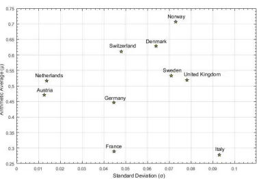
as ‘Theσ−µplane’, which is illustrated in Figure 1 and shows the standard deviationσ(on the
horizontal axis) and the meanµ(on the vertical axis) of ten European countries with respect
to the data of the 2017 World Happiness Report (WHR) (Helliwell et al., 2017) that will be detailed in Section4.
Moreover, one can define aσ−µPareto dominance relation on the set of unitsI as follows:
for alli, i′ ∈I, unitiis Pareto dominating uniti′ ifµi ≥µi′ and σi ≤σi′, with at least one of
the two inequalities being strict. A uniti∈I isσ−µPareto efficient if there is no other unit
dominating it. The set of all Pareto efficient units constitutes the Pareto frontier. A concept stricter than σ −µ Pareto efficiency is the σ−µ Pareto-Koopmans efficiency (Charnes and
Cooper,1962). A uniti∈Iisσ−µPareto-Koopmans efficient if there is no convex combination
of µi′ and σi′ of the remaining units, i′ 6= i, with a mean value µ that is not smaller, and a
standard deviationσ that is not greater, with at least one of these inequalities being strict.
Formally, a unit i ∈ I is σ−µ Pareto-Koopmans efficient if for all vectors [λi′, i′ 6= i], with
X
i′6=i
λi′µi′ > µi and
X
i′6=i
λi′σi′ ≤σi (3)
X
i′6=i
λi′µi′ ≥µi and
X
i′6=i
[image:14.612.117.496.241.503.2]λi′σi′ > σi. (4)
Figure 1: Theσ−µplane.
Unitsi∈Iare plotted on the plane with coordinates (σi,µi). Theσ−µanalysis hereby
presented concerns ten EU countries evaluated with respect to the data of the 2017 World Happiness Report (WHR) (Helliwell et al.,2017) as explained in Section 4.
The set of all σ−µ Pareto-Koopmans efficient units constitutes theσ−µPareto-Koopmans
frontier. The membership of a uniti ∈ I to the Pareto-Koopmans efficiency frontier can be
verified with a direct or an indirect procedure described below.
The direct procedure verifies that there exists no unit -obtained as linear combination of meanµi′ and standard deviationσi′- dominating uniti. This is obtained by considering the
ε∗i =Maxε s.t. X
i′6=i
λi′µi′ >µi+ε
X
i′6=i
λi′σi′ 6σi−ε
λ′i>0, ∀i′ 6=i
X
i′6=i
λi′ = 1
where a unit,i, isσ−µPareto-Koopmans efficient ifε∗i 60. The indirect procedure to test the
σ−µPareto-Koopmans efficiency requires to consider the following LP problem:
δ∗i =Maxδ s.t.
αµi−βσi>αµi′ −βσi′+δ, ∀i′ 6=i
α, β>0
α+β = 1
(5)
which can be interpreted as follows. An evaluationαµi′−βσi′, withα, β >0andα+β= 1, is
assigned to all unitsi′ ∈I. The non-negative coefficientαfor the meanµi′ and the non-positive
coefficientβfor the standard deviationσi′ are coherent with the idea thatµi′ is intended to be
maximised andσi′ is intended to be minimised. Therefore, ideally, the greaterαµi′−βσi′, the
better the uniti′performs with respect toµi′ and σi′. The LP problem verifies whether a pair
(α, β)exists, for which unit i∈I receives an evaluation that is not worse than the remaining
units, i′ 6= i, that is ifαµi−βσi > αµi′ −βσi′ +δ, ∀i′, with a non-negative value ofδ. This
happens if δi∗ > 0, which, for the units belonging to the σ −µ Pareto-Koopmans efficiency
frontier, represents the margin that can be subtracted from the overall evaluationαµi−βσiof unitimaintaining the maximality of its evaluation with respect to all other unitsi′ 6= i. For
all unitsi∈I that do not belong to theσ−µPareto-Koopmans efficiency frontier, the greater
the absolute value ofδi∗, the greater the margin that has to be added toαµi−βσi, in order to attain the evaluationαµi′−βσi′of the units belonging to theσ−µPareto-Koopmans efficiency
frontier. In this sense, the value ofδ∗i can be interpreted as a measure of efficiency of uniti∈I
with the following characteristics:
• ifδi∗ is non-negative, then unitiis efficient, with higher values of δ∗i indicating greater
efficiency fori,
• ifδ∗i is non-positive, then unitiis inefficient, with higher values of|δ∗
i|indicating greater inefficiency fori.
For this reason, in the following we shall refer toδi∗ as theσ−µPareto-Koopmans efficiency
The following proposition enunciates the equivalence between the direct and the indirect test of theσ−µPareto-Koopmans efficiency.
Proposition 1. δ∗i >0if and only ifε∗i 60
Proof. Let us start by proving that ifδ∗i >0thenε∗i 60.
Ifδi∗>0, then there existsα, β>0, withα+β = 1, for which:
αµi−βσi >αµi′−βσi′ for alli′ 6=i.
Therefore, for allλ= [λi′, i′ 6=i]withλi′ >0, for alli′ 6=i, and P
i′6=i
λi′ = 1, we have:
λi′(αµi−βσi)>λi′(αµi′ −βσi′)for alli′ 6=i (6)
By (6) we can get the following:
X
i′6=i
λi′(αµi−βσi)>
X
i′6=i
λi′(αµi′−βσi′),
and, consequently,
αµi−βσi >α
X
i′6=i
λi′µi′ −β
X
i′6=i
λi′σi′.
This implies that the following condition is not verified with at least one strict inequality:
X
i′6=i
λi′µi′ >µi
X
i′6=i
λi′σi′ 6σi
This amounts to the Pareto-Koopmans efficiency of uniti, so that we have ε∗ ≤ 0. Thus, we proved that ifδ∗i >0, thenε∗i 60. Let us now prove that ifε∗i 60, thenδi∗>0.
For a given unit,i, let us consider the pair(σi, µi)and the two following sets:
• the setP+(σi, µi)of all the pairs(σ, µ)∈R2+Pareto dominating(σi, µi), that is
P+(σi, µi) ={(σ, µ)∈R2+:σ ≤σi andµ≥µi with at least one strict inequality}
• the setP−(σi, µi)given by the convex hull of the pairs(σi′, µi′)withi′ 6=i, that is
P−(σi, µi) =
X
i′6=i
λi′µi′,
X
i′6=i
λi′σi′
:λi′ ≥0for alli′ 6=iand
X
i′6=i
λi′ = 1
.
Let us remind that the condition ε∗i 6 0 implies that (σi, µi) is Pareto-Koopmans efficient. This means that there exists no pair (σ, µ) ∈ R2
(σi′, µi′) ∈ R2+, i′ 6= i that is dominating (σi, µi). As the set of pairs (σ, µ) ∈ R2+ dominat-ing (σi, µi) is P+(σi, µi) and the set of convex combinations of the pairs (σi′, µi′), i′ 6= i, is
P−(σi, µi), the Pareto-Koopmans efficiency of(σi, µi)amounts to the condition thatP+(σi, µi) andP−(σi, µi)are disjoint. Let us point out that bothP+(σi, µi)andP−(σi, µi)are convex sets in R2. Therefore, for the hyperplane separating theorem (see e.g. Boyd and Vandenberghe
(2004), there must be a hyperplane separatingP+(σi, µi)fromP−(σi, µi)in theσ−µspace. In fact, this means that there exists a straight lineαµ−βσ =γ, such that:
αµ−βσ > γ
for all(σ, µ)∈P+(σi, µi), and
αµ−βσ < γ
for all(σ, µ) ∈P−(σi, µi). For contradiction, suppose now thatδ∗i <0. This means that for all
α, β≥0we have
αµi−βσi < αµi′−βσi′
for at least onei′ 6=i. Thus, for allγ ∈R
αµi−βσi > γ
implies
αµi′−βσi′ > γ
for at least onei′6=i. But(σi′, µi′)∈P−(σi, µi)and therefore, there cannot exist any hyperplane
αµ−βσ=γ
separatingP+(σi, µi)from P−(σi, µi). Thus, in this case the pair(σi, µi) is not σ−µ Pareto-Koopmans efficient. So, ifε∗
i 60and, consequently(σi, µi)is efficient, thenδ∗i >0.
Theσ−µPareto-Koopmans efficiencyδ∗
i of uniti∈I refers to theσ−µPareto-Koopmans efficiency frontier. However, for a unit that is quite remote from theσ −µPareto-Koopmans
efficiency frontier, it might not be very meaningful to compare it with units of that frontier, as they could be seen as potentially implausible benchmarks. Instead, it could be useful to compare these remote units with their counterparts that are closer to them in theσ−µplane,
and as such, constitute more realistic benchmarks. This suggests taking into consideration the idea of a sequence of efficiency frontiers considered within the celebrated evolutionary multi-objective optimization algorithm NSGA-II (Deb et al.,2002).
A first sequence ofσ−µefficiency frontiers can be defined by taking into consideration the
Pareto dominance. In this perspective, the set of allσ −µ Pareto-efficient units constitutes
the firstσ−µPareto efficiency frontier, denoted byP F1. RemovingP F1fromIand computing again the σ −µ Pareto efficiency frontier for the remaining units, we get the second σ −µ
The sequence of Pareto efficiency frontiersP F1, P F2, . . . , P Fpbased on the concept of Pareto dominance is used in NSGA-II (Deb et al.,2002). However, for the sake of our analysis, an anal-ogous sequence of efficiency frontiers based on the concept of Pareto-Koopmans dominance seems more appropriate. The idea of a series of Pareto-Koopmans frontiers has been origi-nally introduced by Seiford and Zhu (2003) as “context-dependent” data envelopment analysis. It was developed to show the ‘attractiveness’ or ‘progress’ of each evaluated DMU, according to each frontier in the sequence. The reason being is that the authors assume each efficiency frontier (or ‘level’) to be an alternative ‘evaluation context’ that, measuring the ‘attractive-ness’ of each unit from, greatly facilitates identifying DMUs with outstanding performance, or simply to differentiate between efficient DMUs. In the spirit of their study, we suggest decomposing the set of evaluated DMUs into a sequence of Pareto-Koopmans frontiers that illustrate theσ−µefficient DMUs on each level. We call the efficiency frontiers of this new
se-quence firstσ−µPareto-Koopmans efficiency frontier, denoted byP KF1, secondσ−µ Pareto-Koopmans efficiency frontier, denoted by P KF2, and so on and so forth. Let us denote by PKF ={P KF1, . . . , P KFp}the set of all the σ−µPareto-Koopmans efficiency frontiers. For
each uniti∈I, and for eachσ−µPareto-Koopmans efficiency frontierP KFk∈PKF, we can define a ‘local’σ−µPareto-Koopmans efficiencyδikwith respect toP KFk as follows:
δik =Maxδ
s.t.
αµi−βσi >αµi′−βσi′ +δ, ∀i′∈I\
k−1[
h=1
P KFh
α, β >0
α+β= 1
(7)
The above LP problem verifies whether there exists a pair(α, β), for which uniti∈I receives
an evaluation αµi −βσi which is not worse than the analogous evaluation of the rest of the unitsi′ ∈I \Sk−1h=1P KFh, that is, all the unitsi′ belonging to thekthσ−µPareto-Koopmans efficiency frontier, or to a better σ−µ Pareto-Koopmans efficiency frontier. This happens if δik >0. Instead, ifδik <0, then unit ibelongs to aσ−µPareto-Koopmans efficiency frontier worse than P KFk, that is, i ∈ P KFh with h = k+ 1, . . . , p. The interpretation of δik with respect to thekthσ−µPareto-Koopmans efficiency frontier is analogous to the interpretation
ofδi∗ with respect to the overallσ−µPareto-Koopmans efficiency frontier. More precisely, for
the units in thekthσ−µPareto-Koopmans efficiency frontier or better,δik>0represents the margin that can be subtracted from the overall evaluationαµi−βσiof unitimaintaining an evaluation that is superior to all units in thekth σ−µPareto-Koopmans efficiency frontier or
worse. Instead, for all unitsi∈Ibelonging to thekthσ−µPareto-Koopmans efficiency frontier or worse, the absolute value ofδi∗<0represents the margin that has to be added toαµi−βσi, in order to obtain the same evaluation of at least one unit belonging to k-th σ −µ
Pareto-Koopmans efficiency frontier or better. Therefore, asδ∗
i constitutes an efficiency measure with respect to the overallσ−µPareto-Koopmans efficiency frontier (that, in fact, corresponds to
respect to the overall kth σ −µ Pareto-Koopmans efficiency frontier. For this reason, in the
following we shall refer toδikasσ−µPareto-Koopmans efficiency of unitiwith respect to the
kthfrontier.
The following proposition gives a simple, yet useful result with respect to the σ−µ
Pareto-Koopmans efficiency corresponding to thekthfrontier.
Proposition 2. Theσ−µPareto-Koopmans efficiency respects theσ−µPareto dominance,
that is, for alli, i′∈I ifµ
i >µi′ andσi6σi′, thenδik >δi′kfor anyk= 1, . . . , p.
Proof. As µi > µi′ and σi 6 σi′, αµi −βσi > αµi′ −βσi′ for all α, β > 0 with α +β = 1.
Consequently,
αµi′−βσi′ >αµi′′−βσi′′+δ
implies
αµi−βσi>αµi′′−βσi′′+δ
for anyi′′ ∈I and anyδ∈R. Therefore,
αµi′ −βσi′ >αµi′′−βσi′′+δi′k, ∀i′′∈I\
k−1[
h=1
P KFh
implies
αµi−βσi >αµi′′−βσi′′+δi′k, ∀i′′∈I\
k−1[
h=1
P KFh.
Consequently, sinceδikis the maximumδsatisfying
αµi−βσi>αµi′′−βσi′′+δ, ∀i′′∈I\
k−1[
h=1
P KFh,
we have to conclude thatδik >δi′k.
Augmenting the above analysis and the classic concept of context-dependent DEA, we may proceed to a more holistic evaluation as follows. To all unitsi ∈ I, we can assign an overall,
‘global’σ−µPareto-Koopmans efficiency score, denoted bysmi, that reflects its efficiency with respect to all frontiers fromPKF, as follows:
smi = p
X
k=1
δik. (8)
The following corollary of Proposition 2 ensures that overallσ−µPareto - Koopmans efficiency scoresmi respects theσ−µPareto dominance.
Proposition 3. For alli, i′∈I ifµi >µi′ andσi6σi′, thensmik >smi′k.
Conse-quently, we have
smi = p
X
k=1
δik> p
X
k=1
δi′k=smi′.
In the following we supply some remarks related to the application of our approach in real life problems. As usual for the other indicators of SMAA, the integrals defining the mean valueµi and the standard deviationσi,i∈I, can be approximated by numerical methods or via the use of a Monte-Carlo simulation, which, as noted in Daraio and Simar (2005,2007a) (as applied to the computation of the m, ora-order efficiency measures), is a usual and convenient way
to avoid numerical integration. In fact, as the authors acknowledge (Daraio and Simar,2005, p.103), “the quality of the approximation can be tuned” by increasing the number of simulations (in our particular case, this would refer to the number of random draws of the weight vectors). Therefore, using a random sampling ofq vectors of weights - withq being a relatively large
number; for instance, following the suggestions of Tervonen and Lahdelma (2007), q could
equal 10,000- we may approximate the two parameters of interest. The q random extracted
weight vectors wh = [w1h, . . . , wmh], h = 1, . . . , q can be collected in the following m×q RW matrix: RW m×q =
w11 w12 · · · w1q
w21 w22 · · · w2q ... ... · · · ... wm1 wm2 · · · wmq
Using the weight vector matrixRW, a composite indicatorCI(xi,wh)can be computed for each
uniti∈I and each weight vectorwh, and the obtained results can be ordered in the following n×qmatrixCIshown below:
CI n×q=
CI(x1,w1) CI(x1,w2) · · · CI(x1,wq) CI(x2,w1) CI(x2,w2) . . . CI(x2,wq)
... ... · · · ...
CI(xn,w1) CI(xn,w2) · · · C(xn,wq)
Using the values collected inCI, for each uniti∈I one can compute the approximated values
e
µiand eσifor the meanµiand the standard deviationσi as follows:
e
µi= 1
q
q
X
h=1
CI(xi,wh),
e
σi=
v u u t1 q q X h=1
It is worth noting that, when it comes to real-world applications, the existence of outliers is a constant struggle and an issue that appears more often than not (Hawkins, 1980). The presence of outliers in a working data set could seriously impact the obtained estimators of local and global efficiency measures respectively. In such a case, the preceded analysis could be greatly benefited by established robust frontier techniques (e.g. see, among others, the studies of Simar and Wilson,1998; Daraio and Simar,2005,2007b). In this study we will consider the use of ‘partial’ frontier techniques, such as them-order frontiers (Cazals et al.,2002; Daraio
and Simar, 2005) to obtain robust estimators for the local and global σ −µ efficiencies. An
extended discussion and application is presented in sub-section 5.1.
Last but not least, before concluding this section, let us comment on the concept of efficiency we are proposing, comparing it with other efficiency measures proposed in the literature. First, note that we are considering a non-parametric frontier approach for the “production set” Ψ of pairs (σ, µ). In fact, in our approach, Ψ is the set of all pairs (σ, µ) obtained as convex combination of pairs(σi, µi), i= 1, . . . , n, that is
Ψ =
( n X
i=1
λiµi, n
X
i=1
λiσi
!
:λi ≥0, i= 1, . . . , n, and n
X
i=1
λi= 1
)
,
which has the following efficient frontier:
b
Ψ =(σ, µ) : there is no(σ′, µ′)∈Ψsuch that(σ′, µ′)6= (σ, µ), σ′ ≤σ andµ′≥µ .
The Pareto-Koopmans efficiencyδi∗we compute can be interpreted as a distance from the
effi-cient frontierΨb. Indeed, we can imagine to scalarize the vectors(σ, µ)introducing the scalar-ization functionFα,β(σ, µ) =αµ−βσ, α, β≥0, α+β = 1,, measuring the distanceD
(σ, µ),Ψb between(σi, µi), i= 1, . . . , n,and the efficient frontierΨb as:
D(σi, µi),Ψb
=min(σ′,µ′)∈ΨbFα,β(σi, µi)−Fα,β(σ′, µ′),
and, finally, taking into account all the feasible pairs(α, β)we get:
δ∗i =minα,β≥0,α+β=1D(σi, µi),Ψb
.
In fact, practically all the measures of efficiency proposed in the literature can be expressed in terms of a distance from a frontier. In this sense, the Debreu-Farrell efficiency measure (Debreu,1951; Farrell,1957) gives the radial distance of the point with respect to the efficiency frontier, which in the context of the σ−µ−efficiency analysis amounts to the following two efficiency measures:
• aµ-oriented efficiency measure that provides the valueθµ(σi, µi), which shall be multi-plied by the averageµito permit unitito become Pareto-Koopmansσ−µ−efficient, that is:
so that, the smallerθµ(σi, µi), the more efficient is unitithat can be considered Pareto-Koopmans efficient ifθµ(σi, µi) = 1;
• aσ-oriented efficiency measure that provides the valueθσ(σi, µi)to be multiplied by the standard deviationσi to permit unit ibecoming Pareto-Koopmansσ−µ−efficient, that is:
θσ(σi, µi) =max{θ|(θσi, µi)∈Ψb}, (10)
so that, the greaterθσ(σi, µi), the more efficient is unitithat can be considered Pareto-Koopmans efficient ifθσ(σi, µi) = 1.
Of course, in such case the LP problem formulation for theµandσ-oriented efficiency measures
(eq.9&10respectively) would be the following:
θiµ=Maxθ s.t.
θµi ≤ n
X
j=1
λjµj
σi ≥ n
X
j=1
λjσj
λj >0
X
λj = 1
(11a)
θσi =Minθ s.t.
µi≤ n
X
j=1
λjµj
θσi ≥ n
X
j=1
λjσj
λj >0
X
λj = 1
(11b)
while, in the spirit of Andersen and Petersen (1993), one could compute the ‘super-efficiency’ of each unit not only with respect to the first, but with respect to each Pareto-Koopmans frontier in the sequence (e.g. ‘lifting’ each time the units lying on a PKF from the constraints and re-computing the LP formulation). This would permit to have an efficiency measure in the[0,1] space for local efficiencies, and in the [0,∞) space for global efficiencies. Yet, the drawback associated with these measures of efficiency is that, in our proposed model, we consider a twofold kind of a trade-off betweenµandσ(see Section6for a discussion of this point) that is
hereby lost.
4
The
σ
-
µ
efficiency analysis step by step: A didactic example
The present section illustrates the application ofσ−µefficiency analysis with a concise
France, Germany, Italy, Netherlands, Norway, Sweden, Switzerland and United Kingdom) for the latest available year (data regarding the year 2016) to be evaluated throughσ−µefficiency
analysis. For the sake of simplicity, we only consider three of the six key variables, and more precisely, GDP per capita, Social support and Perceptions of corruption. We report these in Table 1.
Normalization is an essential part of data aggregation to avoid adding-up “apples and
or-anges” (OECD, 2008, p.27). The reason being is that indicators often come in a variety of
ranges or scales that might render them incomparable in the stage of aggregation (Freuden-berg,2003). According to the author, the most common approach is standardization due to its desirable characteristics that we forthwith quote:
It converts all variables to a common scale and assumes a "normal" distribution; it has an average of zero, meaning that it avoids introducing aggregation distortions stemming from dif-ferences in variable means. In the other approaches, the scaling factor is the range of the distri-bution, rather than the standard deviation, which means that extreme values can have a large
effect on the composite indicator(Freudenberg,2003, p.11).
We start by standardizing the raw data reported in Table 1. As Booysen (2002, p.123) argues, “standard scores can be further adjusted if calculations yield awkward values”. Adjustment of these values is in fact a reasonable exercise. De Muro et al. (2011) choose to adjust these values around the range[70,130]with the value of a100being a good reference point (mean around which the standard deviations will revolve). In their spirit, Greco et al. (2018a, see online Appendix A.2) choose a different adjustment range for the standardized values. In particular, they set it to[0,1], with0.5being the mean around which the standard deviations will revolve. Values falling outside this range (3 standard deviations away from the mean) will be replaced with the lower or upper bound accordingly, as they could generally be considered extreme given that within this range lie 99.73% of the values in the case of a normal distribution, and 89% of the values in the case of any distribution (Chebyshev’s inequality). We will hereby adopt this normalization that we describe in the following:
Let us denote byyij,i∈I, j ∈J the raw value assumed for unitiwith respect to dimensionj. For each dimensionj∈J, the mean valueMj and the standard deviationsj can be computed as follows:
Mj =
Pn i=1yij
n ,
sj =
rPn
i=1(yij −Mj)2
n .
Using the mean Mj and the standard deviation sj, for each i ∈ I and j ∈ J we obtain the
z-score :
zij =
yij −Mj
sj
Table 1: Raw and normalized values of the considered dimensions.
Raw Data Normalized values
Country Log of GDP Social Perceptions of Country Log of GDP Social Corruption
per capita support corruption per capita support free
Austria 10.69 0.93 0.52 Austria 0.48 0.49 0.44
Denmark 10.68 0.95 0.21 Denmark 0.47 0.70 0.71
France 10.54 0.88 0.62 France 0.33 0.18 0.35
Germany 10.70 0.91 0.45 Germany 0.49 0.34 0.51
Italy 10.43 0.93 0.90 Italy 0.23 0.50 0.11
Netherlands 10.76 0.93 0.43 Netherlands 0.54 0.49 0.52
Norway 11.07 0.96 0.41 Norway 0.84 0.74 0.54
Sweden 10.74 0.91 0.25 Sweden 0.53 0.38 0.68
Switzerland 10.92 0.93 0.30 Switzerland 0.70 0.50 0.63
United Kingdom 10.57 0.95 0.46 United Kingdom 0.37 0.70 0.50
Average 10.71 0.93 0.46
Standard Deviation 0.17 0.02 0.19
Data: 2017 World Happiness Report (WHR), obtained from: http://worldhappiness.report/ed/2017/. The data regard the year 2016. The detailed description and the sources of the considered dimensions can be found in Helliwell et al. (2017, p.17).
Finally, we compute the normalized valuesxij as follows:
xij =
0, ifyij 6Mj−3sj
0.5 +zij
6 , ifMj −3sj < yij < Mj+ 3sj 1, ifyij >Mj+ 3sj
The normalization is applicable to positively-oriented dimensions, that is, dimensions for which the greater the raw value the better (e.g. GDP per capita and Social Support). Instead, for negatively-oriented dimensions, for which the greater the raw value the worse for a unit’s per-formance (e.g. Perception of corruption), the normalization is formulated as follows:
xij =
0, ifyij >Mj+ 3sj
0.5−zij
6 , ifMj −3sj < yij < Mj+ 3sj 1, ifyij 6Mj−3sj
Let us explain the general idea behind this normalization. Let us denote byyj∗andy∗j the worst and best values respectively that are taken under consideration, such that, beyond these values we consider the evaluationyij with respect to dimensionj ∈I an outlier. This means that, if the dimensionj is positively-oriented, thenyj∗ < yj∗, and all the valuesyij ≤yi∗ are assigned a valuexij = 0, as well as all the valuesyij ≥yi∗ are assigned a valuexij = 1. Instead, if the dimension jis negatively-oriented, then yj∗ > y∗j, and all the valuesyij ≤ yi∗ are assigned a value of xij = 1, while all the values yij ≥ yi∗ are assigned a value of xij = 0. We consider as outlier a value yij which extendsγ ×sj beyond/above the meanMj, and, since we hereby fixedγ = 3(though, of course, other values ofγcan be assigned according to the nature of the
problem), this amounts to yj∗ = Mj −3sj and y∗j = Mj + 3sj ifj is positively-oriented, and
yj∗ =Mj+ 3sj andx∗j =Mj−3sj ifjis negatively-oriented. Then, in case the value ofyij lies between the values ofyj∗ andy∗j, it can be normalized as follows (where ±means +in casej is positively-oriented and−in casejis negatively oriented, and vice versa for∓):
xij =
yij −yj∗
y∗j −yj∗
= yij−(Mj∓3sj) (Mj±3sj)−(Mj∓3sj)
=
yij−Mj ±3sj
±6sj
= 0.5±yij−Mj
6sj
= 0.5± zij
6sj
.
If the value of yij lies outside the interval ofyj∗ andyj∗, then the normalized value ofyij (i.e.
xij) is either 0 or 1 as explained above.
With respect to the creation of the weight vector matrixRW, in this didactic example we
con-sider the following two scenarios, wherewGDP, wSoc, wCorrdenote weights for GDP per capita, Social support and Perception of corruption respectively:
the set of feasible weight vectors is
W={[wGDP, wSoc, wCorr] :wGDP >0, wSoc >0, wCorr>0, wGDP +wSoc+wCorr = 1};
• Scenario 2: Social support is more important than Perception of corruption that in turn
is more important than GDP per capita, so that the set of feasible weight vectors is
W={[wGDP, wSoc, wCorr] :wSoc >wCorr>wGDP >0, wGDP +wSoc+wCorr= 1}.
For both scenarios, a set of 10,000 weight vectorswh,h= 1, . . . ,10,000, was randomly sampled from a uniform distribution on the feasible set of weight vectorsWand collected in the matrix RW = [wjh, j = 1,2,3, h = 1, . . . ,10,000]. The weight vectors from RW and the normalized
valuesxij,i= 1, . . . ,10, j= 1,2,3,are then used to compute the composite indicators:
CI(xi,wh) =wGDPxi,GDP+wSocxi,Soc+wCorrxi,Corr, h= 1, . . . ,10,000.
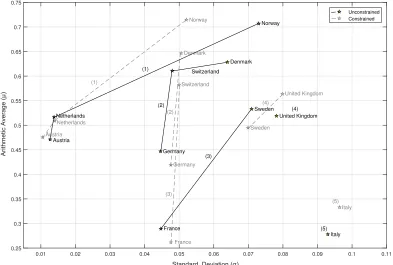
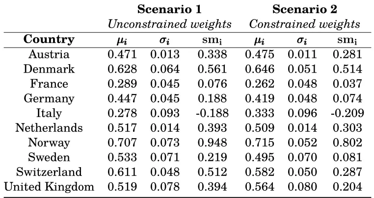
Using the values CI(xi,wh), i = 1, . . . ,10, h = 1, . . . ,10,000, the approximation of the mean valueµei and the standard deviationσei of composite indicators were calculated for each con-sidered country. For the sake of simplicity, we refer to them asµi andσi, respectively. These two measures are reported for both considered scenarios in Table 2 and plotted, along with the respective Pareto-Koopmans frontiers, on Figure 2.
The σ−µPareto-Koopmans local efficiencies δik of the considered countries with respect to the differentσ−µPareto-Koopmans efficiency frontiers are given in Table 3. In both
exam-ined scenarios, theσ−µPareto-Koopmans family of frontiers consists of five frontiers. For the
first scenario, that without a definite ranking of importance for the considered dimensions, the five frontiers are the following: P KF1 = {Norway, the Netherlands, Austria} , P KF2 =
{Denmark, Switzerland, Germany},P KF3 = {Sweden, France},P F K4 = {United Kindom},
P KF5 ={Italy}. In the second scenario, theσ−µPareto-Koopmans frontiers remain the same with the exceptions of Switzerland, that was in the secondσ−µPareto-Koopmans efficiency
frontier in the first scenario but descended to the third frontier in the second scenario. Simi-larly, Sweden, which was in the third frontier in the first scenario has been now descended to the fourth frontier.
In terms of their overall, global efficiencies (smi), Norway presents the highest score, while the second highest score is attributed to Denmark in both scenarios. It is worthwhile to ob-serve that Denmark is not in the first σ−µPareto-Koopmans efficiency frontier, which,
Figure 2: Illustrative example of theσ−µplane in the two scenarios considered.
Black colour representsσ−µefficiency analysis output in the unconstrained case (i.e. scenario 1),
while grey colour representsσ−µefficiency analysis output in the constrained case (i.e. scenario 2). Numbers in parentheses denote respectiveσ−µPareto-Koopmans efficiency frontier (P KFi).
0.01 0.02 0.03 0.04 0.05 0.06 0.07 0.08 0.09 0.1 0.11 0.25 0.3 0.35 0.4 0.45 0.5 0.55 0.6 0.65 0.7 0.75 Germany France Netherlands Italy United Kingdom Switzerland Austria Sweden Norway Denmark Germany France Netherlands Italy United Kingdom Switzerland Austria Sweden Norway Denmark Unconstrained Constrained (1) (2) (3) (4) (5) (1) (2) (3) (4) (5)
score as to the first two frontiers, which is reasonable given that it lies on a higher fron-tier (δAustria1 = 0.001,δDenmark1 = −0.012,δAustria2 = 0.032,δDenmark2 = 0.018); still, Denmark is ‘catching-up’ and, in fact, surpassing Austria by being more efficient with respect to the remaining three frontiers and, in particular, boasting almost twice the Austria’s efficiency (δAustria3 = 0.047,δDenmark3 = 0.095,δAustria4 = 0.065,δDenmark4 = 0.11,δAustria5 = 0.193,δDenmark5 = 0.35). Understandably, the same applies also when it comes to the comparison of Denmark and the Netherlands, as well as Switzerland and the Netherlands or Austria. Of course, as proven in proposition 3, the same could not apply to Germany, which, despite the fact that it shares the frontier with Switzerland and Denmark, it is dominated by both Austria and the Netherlands in both parameters. Additionally, let us also observe that in both scenarios Italy is the only country for which the efficiency score,smi, is negative. On the other hand, Italy is also the only country in the worst efficiency frontier.
Observe, finally, that the σ−µ efficiency analysis described above can be interpreted as
the application of a multiple criteria decision aid method to evaluate the attractiveness of the considered countries. In this perspective this procedure can be seen as a new method in the SMAA family. We call this new methodσ−µ−SMAA (for another method taking into account
Table 2: Evaluating the units withσ−µunder the two alternative scenarios.
Scenario 1
Scenario 2
Unconstrained weights
Constrained weights
Country
µ
µ
µ
iiiσ
σ
σ
iiism
iµ
µ
µ
iiiσ
σ
σ
iiism
iAustria
0.471 0.013
0.338
0.475 0.011
0.281
Denmark
0.628 0.064
0.561
0.646 0.051
0.514
France
0.289 0.045
0.076
0.262 0.048
0.037
Germany
0.447 0.