Libration Points in the R3BP with a Triaxial Rigid Body as the Smaller Primary and a Variable Mass Infinitesimal Bod

ISSN Online: 2161-4725 ISSN Print: 2161-4717

DOI: 10.4236/ijaa.2019.91003 Mar. 5, 2019 21 International Journal of Astronomy and Astrophysics

Libration Points in the R3BP with a Triaxial

Rigid Body as the Smaller Primary and a

Variable Mass Infinitesimal Body

M. R. Hassan

1

_{, Sweta Kumari}

2

_{, R. R. Thapa}

3

_{, Md. Aminul Hassan}

4 1_{Department of Mathematics, S. M. College, T. M. Bhagalpur University, Bhagalpur, India} 2_{T. M. Bhagalpur University, Bhagalpur, India}

3_{Department of Mathematics, P. G. Campus, Tribhuvan University, Biratnagar, Nepal} 4_{GTE, Bangalore, India}

Abstract

The paper deals with the existence of the coplanar libration points in the re-stricted three-body problem when the smaller primary is a triaxial rigid body and the infinitesimal body is of variable mass. Following small parameter method, the coordinates of collinear libration points are established whereas the coordinates of triangular libration points are established by classical me-thod. It is found that the mass reduction factor has small effect but triaxiality parameters of the smaller primary have great effects on the coordinates of the libration points.

Keywords

Restricted Three-Body Problem, Jean’s Law, Space-Time Transformation, Triaxiality, Mass Reduction Factors, Libration Points

1. Introduction

Restricted three-body problem with variable mass has an important role in ce-lestial mechanics. The phenomenon of isotropic radiation or absorption in stars was studied by the leading scientists to formulate the restricted three-body problem with variable mass. The two body problem with variable mass was stu-died by Jeans [1] regarding the evaluation of binary system. Meshcherskii [2] assumed that the mass is ejected isotropically from the two body system at very high velocities and is lost to the system. He examined the change in orbits, the variation in angular momentum and the energy of the system. Shrivastava and

How to cite this paper: Hassan, M.R., Kumari, S., Thapa, R.R. and Hassan, Md.A. (2019) Libration Points in the R3BP with a Triaxial Rigid Body as the Smaller Primary and a Variable Mass Infinitesimal Body. International Journal of Astronomy and Astrophysics, 9, 21-38.

https://doi.org/10.4236/ijaa.2019.91003

Received: November 8, 2018 Accepted: March 2, 2019 Published: March 5, 2019

Copyright © 2019 by author(s) and Scientific Research Publishing Inc. This work is licensed under the Creative Commons Attribution International License (CC BY 4.0).

http://creativecommons.org/licenses/by/4.0/

DOI: 10.4236/ijaa.2019.91003 22 International Journal of Astronomy and Astrophysics Ishwar [3] derived the equations of motion of the circular restricted three-body problem with variable mass with the assumption that the mass of the infinite-simal body varies with respect to time. Singh and Ishwar [4] showed the effect of perturbation due to oblateness on the existence and stability of the triangular li-bration points in the restricted three-body problem.

Das et al. [5] developed the equations of motion of elliptic restricted three-body problem with variable mass. Lukyanov [6] discussed the stability of libration points in the restricted three-body problem with variable mass. He has found that for any set of parameters, all the libration points in the problem (Collinear, Triangular) are stable with respect to the conditions considered by the Mesh-cherskii’s space-time transformation. El Shaboury [7] had established the equa-tions of motion of elliptic restricted three-body problem (ER3BP) with variable mass with two triaxial rigid primaries. He has applied the Jeans law, Nechvili’s transformation and space-time transformation given by Meshcherskii in a spe-cial case.

Singh et al. [8] have discussed the non-linear stability of libration points in the restricted three-body problem with variable mass. They have found that in non-linear sense, collinear points are unstable for all mass ratios and the trian-gular points are stable in the range of linear stability except for three mass ratios depending upon the mass variation parameter

β

governed by Jean’s law. Has-san et al. [9] studied the existence of libration points with variable mass in the R3BP when the smaller primary is an oblate spheroid. They found that Jacobi constant C= =1,C 2 _{shows no effect in the position of libration points, but for}

3

C= _{, slight shifting of libration points is found due to oblateness only not due} to the mass reduction factor α .

In present work, we have established coordinates of five libration points

(

1,2,3,4,5

)

i

L i= _{in the R3BP with variable mass when smaller primary is a} tri-axial rigid body by small parameter method [10] and the method used by Hassan et al. [9].

2. Equations of Motion

Let the two primaries of non-dimensional masses

µ

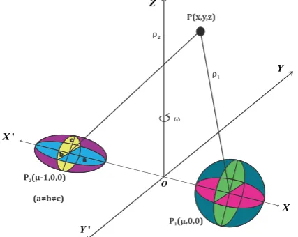
and 1−µ be moving on the circular orbits about their centre of mass. In Figure 1, we consider a bary-centric coordinate system

(

O XYZ,

)

rotating relative to the inertial frame with angular velocity ω_{. The line joining the centers of} P₁ and P2 of the

primaries is considered as the x-axis and a line lying on the plane of motion and perpendicular to the x-axis and through the centre of mass; as the y-axis and a line through the centre of mass and perpendicular to the plane of mo-tion as the z-axis. Let

(

µ

,0,0

)

and

(

µ

−1,0,0

)

respectively be the coordi-nates of P1 and P2 and

(

x y z, ,

)

be the coordinates of the infinitesimal

body of variable mass m at P.

[image:3.595.266.480.74.244.2]

DOI: 10.4236/ijaa.2019.91003 23 International Journal of Astronomy and Astrophysics

Figure 1. Configuration of R3BP when smaller primary is triaxial.

(

)

_{

₍

₎

_}

(

)

{

}

1 2

1 2 2 1 2 1

3 3 5 5

1 2 2 2

2 2

1 2 1 2

7 2

d d d d

3 2

1 3 _{ˆ ˆ}

2

15 _,

2

m

t t

Gm yj zk

y z

µ σ σ

µ µ _{µ σ σ σ}

ρ ρ ρ ρ

µ σ σ σ

ρ

 

 

 

−  −

= − _ + + + − +





− − + _

 r

ρ ρ ρ

ρ

(1)

the differential operators are given by the relations

d _and d dt t dt t

∂ ∂

= + × = + ×

∂ ∂

r r _r

ω ω

(

)

(

)

(

)

1 2

2 2 2 2

2

1 2 1 2 2 2

ˆ ˆ ˆ

ˆ ˆ _, ˆ ˆ _{, 1} ˆ ˆ _, 3

1 2 , , ,

2 5 5

xi yj zk x i yj zk x i yj zk

a c b c

R R

µ µ

ω σ σ σ σ

= + + = − + + = − + + +

− −

= + − = =

r ρ ρ

(2)

where a b c, , are the semi-axes of the triaxial rigid body, R is the dimensional distance between the centre of the primaries. Thus using Equation (2) in (1), we get

(

)

(

)

(

)

_{

₍

₎

_}

(

)

{

}

2

1 2 2 2

1 2 2 1 2 1 2

3 3 5 7

1 2 2 2

1 2 1

5 2

ˆ ˆ 2

3 2

1 15

2 2

3 _{ˆ ˆ .}

m m m m xi yj

Gm y z

yj zk

ω µ σ σ

µ µ _{µ σ σ σ}

ρ ρ ρ ρ

µ σ σ σ

ρ

+ + × + × − +

−  −

= − _ + + − − +





+ − + _



r r r r

   ω ω

ρ ρ ρ ρ

(

)

{

}

(

)

{

}

(

)

(

)

{

(

)

}

(

)

{

}

2

2

1 2 1 2 2 1 2 1

3 3 5 5

1 2 2 2

2 2

1 2 1 2

7 2

ˆ 2

ˆ ˆ

2

1 3 ₂ 3 _{ˆ ˆ}

2

15 _.

2

mx m x y m y m x i

my m y x m x m y j mz mz k

Gm yj zk

y z

ω ω ω

ω ω ω

µ µ µ _{σ σ} µ _{σ σ σ}

ρ ρ ρ ρ

µ σ σ σ

ρ

⇒ + − − −

+ + + + − + +

 −

= _− − − − − − +





+ − + _



   

     

ρ ρ ρ

ρ

(3)

DOI: 10.4236/ijaa.2019.91003 24 International Journal of Astronomy and Astrophysics written as:

(

)

(

)

1 2 , 1 2 , 1 _, m U

x x y x

m m x

m U

y y x y

m m y

m U

z z

m m z

ω ω ω ω ∂ + − + = − ∂ ∂ + + − = − ∂ ∂ + = ∂            (4) where

(

)

(

)

{

(

)

2 2

}

2 _{1 2 1}

1 2

2 2

3 5

1 2 2 2

3 2

1 _,

2 2 2

y z

m

U

ω

x y m

µ

µ

µ σ σ

µ σ σ

σ

ρ

ρ

ρ

ρ

 _{− −} − + 

 

= − + − + − −

 

  (5)

(

)(

)

(

)

(

)(

)

(

)(

)

(

)

(

)

(

)

(

)

(

)

1 2 2

3 3 5

1 2 2

2 2

1 2 1

7 7

2 2

3 2

1 2 1 2

2 1

3 3 5 7 7

1 2 2 2 2

3 3

1 2

1 1 3 2 1

1

2

15 1 15 1

,

2 2

1 3 2 15 15

1

2 2 2

and

1 3 2

1

x x x

U _x

m x

x y x z

y y y yz

U _y y

m y

z

U z

m z

µ µ µ µ µ σ σ µ

ω

ρ ρ ρ

µ σ σ µ µσ µ

ρ ρ

µ µ µ σ σ µ σ σ µσ

ω

ρ ρ ρ ρ ρ

µ µ µ

ρ ρ − − − − − − − ∂ − = − − − ∂ − − − − − + + − − − ∂ − = − − − + + ∂ − ∂ − = − − + ∂

(

)

(

)

2 3

1 2 1 2 1

5 7 7

2 2 2

15 15 _.

2 2 2

z y z z

σ σ µ σ σ µσ

ρ ρ ρ

− −

+ +

(6)

By Jeans law, the variation of mass of the infinitesimal body is given by

1

d _{. ., ,} d

n n

m _{m i e} m _m

t α m α

−

= − = − (7)

where α is a constant and the value of exponent n∈

[

0.4,4.4

]

for the stars of the main sequence (from Observational facts).

Let us introduce Meshcherskii’s space time transformations [2] as:

1 1 2 2

0

, , , d d , , where 1,

q q q k

q q

x y z t

m

r r

m

ξγ ηγ ζ γ γ τ

ρ γ ρ γ γ

− − − −

− −

= = = =

= = = < (8)

0

m is the mass of the infinitesimal body when t=0 and τ is the pseudo time. From Equation (7) and Equation (8), we get

1

d _,

dt n

γ _{= −βγ} − ₍₉₎

where 1

0n constant

m

β α

₌ − _{= .}

Differentiating x y z, , with respect to t twice and using fourth equation of (8), we get

(

)

(

)

(

)

(

)

(

)

(

)

1 1 1

2 1 2 2 2

2 1 2 2 2

2 1 2 2 2

, , ,

2 1 ,

2 1 ,

2 1 ,

k q n q

k q n q

k q n q

k q n k q n q

k q n k q n q

k q n k q n q

x q

y q

z q

x q k q n q

y q k q n q

z q k q n q

ξ γ β ξγ

η γ β ηγ

ζ γ β ζγ

ξ γ βξ γ β ξ γ

η γ βη γ β η γ

ζ γ βζ γ β ζ γ

DOI: 10.4236/ijaa.2019.91003 25 International Journal of Astronomy and Astrophysics where dot

( )

 represents differentiation with respect to real time t and prime

( )

' represents the differentiation with respect to pseudotime τ _.

Also,

(

)

1

1 1 1 1

0 0 i.e., .

n

n n n n

m _{m m m} m

m α α γ α γ m βγ

−

− − − −

= − = − = − = −

 

Replacing the values of Equation (10) in Equation (4) to obtain

(

)

(

)

( )

(

)

2 1

1 2

2 2 1 1

0

2 1 2

2 1 ,

n k

n k k

q k n q

q k n q q

U q

m

ξ βξ γ ωη γ β ξγ

γ βωηγ ξ − − − − − − − − − ′′+ − − ′ − ′ − − ∂ − − = − ∂

(

)

(

)

( )

(

)

(

)

(

)

( ) 2 1 1 2

2 2 1 1

0

2 2 1

2 1

1 2

0

2 1 2

2 1 ,

2 1 ,

n k

n k k

q k n q

q k n k

n k

q k n q q

U q

m

U

q k n q q

m

η βη γ ωξ γ β ηγ

γ βωξγ

η

γ

ζ βζ γ β ζγ

ζ − − − − − − − − − − − − − − − ′′+ − − ′ + ′ − − ∂ + − = − ∂ ∂ ′′+ − − ′ − − = − ∂ (11) where

(

)

(

)

(

)

1 2

2 2 2 1 2 1 1 3 1

0 3

1 2 2

2 3 1 2 7 1

1 2 1

5 5

2 2

2

1 1

2 2

3 3 _.

2 2

q q q q

q q

U m

r r r

r r

µ σ σ

µ µ

ξ η ω γ γ γ γ

µ σ σ η γ µσ ζ γ

− + + + + + −  − = − _ + + + +   − − −  

As the mass of the infinitesimal body is variable, so only the variational factors but not the non-variational factors should be taken into consideration in the eq-uations of motion of the infinitesimal body. Thus to avoid the non-variational factors, we have

[

]

1 0, 2 1 0, 1 0.4,4.4 , 1

i.e, 0, , 1 and . 2

n k q k n

k q n β α

− − = − − = = ∈

= = = = (12)

Thus the Equations (11) reduced to

2 0 2 0 2 0 1

i.e, 2 ,

4 1 2 , 4 1 _, 4 U m U m U m α

ξ ωη ξ

ξ α

η ωξ η

η α ζ ζ ζ ∂ ′′ ′ − = − + ∂ ∂ ′′ ′ − = − + ∂ ∂ ′′ = − + ∂ (13) where

(

)

(

)

(

)

(

)

{

}

3 3 5

1 2

2 2 2 _{2 2 2}

0 3

1 2 2

7

2 1 2

2

1 2 1

5 2 1 2 1 2 2 3 _, 2 U m

r r r

µ µ µ σ σ

ξ η ω γ γ γ

DOI: 10.4236/ijaa.2019.91003 26 International Journal of Astronomy and Astrophysics

(

)

(

)

(

)

(

)

(

)

(

)

_{

₍

₎

_}

3 3

2 2 2

3 3

0 1 2

5

1 2 ₂

5 2

7

2 1 2

2

1 2 1

7 2 1 1 3 2 2 15 , 2 U

m r r

r

r

µ ξ µ γ µ ξ µ γ γ

ω ξ γ γ

ξ

µ σ σ ξ µ γ γ

γ

µ ξ γ µ γ

γ σ σ η γ− σ ζ γ

− − − + ∂ − = − − ∂ − − + + + − + − +

(

)

(

)

(

)

{

}

(

)

(

)

(

)

{

}

3 3 5

1 2

2 2 2 2

3 3 5

0 1 2 2

7

2 1 2

2

1 2 1

7 2

3 3 5

1 2

2 2 2

3 3 5

0 1 2 2

7

2 1 2

2

1 2 1

7 2

1 3 2

1

2

15 _,

2

1 3 2

1

2

15 _.

2

U

m r r r

r U

m r r r

r

µ η µη µ σ σ η

ω η γ γ γ

η

µη γ σ σ η γ σ ζ γ

µ ζ_γ µζ _γ µ σ σ ζ _γ

ζ

µζ γ σ σ η γ σ ζ γ − − − − ∂ − = − − + ∂ + − + − − ∂ − = − − + ∂ + − + (15)

The Jacobi integral in Meshcherskii’s space is

(

)

(

)

{

(

)

}

(

)

2 2 2

3 3 5

2

1 2

2 2 2 2 2 2 1 2

1 2 1

3

1 2 2

2

2 2 2

2 1 2 2 2 , 4

r r r

C

ξ η ζ

µ σ σ

ω _{ξ η} µ_γ µ_{γ γ σ σ η γ σ ζ γ}

α ξ η ζ

− ′ + ′ + ′  − −  = _ + + + + − + _   + + + + (16)

whereas the Jacobi integral in the rotating frame

(

O XYZ,

)

is

(

)

2 2 2

1 2

2 , , , , , , ,

x +y +z = Ω x y zα ω σ σ +C where

(

)

(

) (

{

)

}

(

)

2

1 2

2 2 2 2

1 2 1

3

1 2 2

2

2 2 2

2 1

2 2

. 4

x y y z

x y z

µ σ σ

ω µ µ _{σ σ σ}

ρ ρ ρ

α

− −

Ω = + + + + − +

+ + +

3. Libration Points

Since in the vicinity of the libration points (Lagrangian points), no translatory motion exists, only vibrational motion exists, hence velocity and acceleration components must vanish at these points i.e., ξ η′= ′=ζ′=ξ′′=η′′=ζ′′=0_.

Thus from Equations (15), we have

(

)

(

)

(

)

(

)

(

)

(

)

{

(

(

)

)

}

3 3

2

2 2 2

3 3

1 2

5

1 2 ₂

5 2 7

2 1 2 1

2

1 2 1

7 2 1 4 3 2 2 15 _0, 2 r r r r

µ ξ µ γ µ ξ µ γ γ

α _{ω ξ γ γ}

µ σ σ ξ µ γ γ

γ

µ γ ξ µ γ γ σ σ η γ σ ζ γ− −

DOI: 10.4236/ijaa.2019.91003 27 International Journal of Astronomy and Astrophysics

(

)

(

)

(

)

{

}

3 3 5

2

1 2

2 _{2 2 2}

3 3 5

1 2 2

5

2 1 2 1

2

1 2 1

7 2

1 3 2

4 2

15 ₀

2

r r r

r

µ η µ σ σ

α _{ω η γ} µη_{γ ηγ}

µη γ σ σ η γ σ ζ γ− −

− −  ₊  _{− − +}     + − + =

(

)

(

)

(

)

{

}

3 3 5

2

1 2

2 2 2

3 3 5

1 2 2

7

2 1 2 1

2

1 2 1

7 2

1 3 2

&

4 2

15 _0.

2

r r r

r

µ ζ µ σ σ

α _{ζ γ} µζ _{γ ζγ}

µζ γ σ σ η γ σ ζ γ− −

− −

 

_{ } − − +

 

+ − + =

For solving the above equations in the rotating frame

(

0,XYZ

)

, we apply the inverse transformation

ξ

=

γ η

x, =

γ ζ

y, =

γ

z _{in the above equations to} get

(

)(

)

(

)

(

)(

)

(

_{) (}

_{

₎

_}

(

)

(

)

_{

₍

₎

_}

(

)

(

)

₍

₎

2 1 2 2

3 3 5

1 2 2

2 2

1 2 1

7 2 2

1 2

2 2 2

1 2 1

3 3 5 7

1 2 2 2

2

1 2 2

1 2

3 3 5 7

1 2 2 2

1 1 3 2 1

4 2

15 1

0, 2

1 3 2 15 _0,

4 2 2

1 3 2 15

4 2 2

x x x

x

x

y z

y y y y

y y z

z z z z

z y

µ µ µ µ µ σ σ µ

α _ω

ρ ρ ρ

µ µ

σ σ σ

ρ

µ µ σ σ

α _ω µ µ _{σ σ σ}

ρ ρ ρ ρ

µ µ σ σ

α µ µ _{σ σ σ}

ρ ρ ρ ρ

− − − + − − +   + − − +     − + + − + = − −   + − − + + − + =     − −   − − + + − +    

{

}

2 1z =0.

(17)

4. Collinear Libration Points

As we know that all the three collinear libration points lie on the x-axis (the line joining the centre of the first and second primary) so y=0,z=0 and hence from Equation (2)

(

)

2

(

)

2

2 2

1 x , 2 x 1

ρ

= −

µ

ρ

= − +

µ

⇒

ρ

₁ = −x

µ ρ

, ₂ = − +x

µ

1.

Thus from Equations (17), we have

(

)(

)

(

)

(

)(

)

2

1 2

2

3 3 5

1 1 3 2 1

0.

4 1 2 1

x x x

x

x x x

µ µ µ µ µ σ σ µ

α _ω

µ µ µ

− − − + − − +

 

+ − − + =

 

− − + − +

  (18)

Let L1

(

ξ1,0,0

)

be the first collinear libration point lying to the left of the

second primary P2

(

µ

−1,0,0 . .,

)

< −i e

ξ

1

µ

1 then ξ1<µ 1 1 0 and 1 0,

ξ µ ξ µ

⇒ − + < − <

(

)

(

)

1 1 x 1 and 1 1 .

ξ µ

µ

ξ µ

ξ µ

⇒ − + = − − + − = − −

Thus from Equation (18),

(

)

(

) (

)

(

)

(

)

2 1 2 2

1 2 2 4

1 1 1

1 3 2

0.

4 1 2 1

µ µ σ σ

α _{ω ξ} µ

ξ µ ξ µ ξ µ

− −

 

+ − − + =

 

− − + − +

  (19)

As ξ1< −µ 1, so let ξ1= − −µ 1 ρ where

ρ

is a very small positive

quan-tity.

DOI: 10.4236/ijaa.2019.91003 28 International Journal of Astronomy and Astrophysics

(

) (

)

(

)

(

)

2 1 2 2

2 2 4

1 3 2

1 0,

4 1 2

µ

µ σ σ

α

_ω

_µ

_ρ

µ

ρ

ρ

ρ

− −  ₊  _{− − − − + =}   − −

  (20)

(

) (

)

(

)

(

)

(

)(

)

2

2 2

2 4 4 2

2

1 2

2 1 1 2 1 2 1

4

3 2 1 0,

α _{ω µ ρ ρ ρ µ ρ µ ρ ρ}

µ σ σ ρ

  + − − + − − − +     + − + = (21)

(

)

(

)

(

)

{

(

)

}

(

)

(

)

2 2 2

2 7 2 6 2 5

2

2 4 3 2

1 2

1 2 1 2

3 2

4 4 4

1 2 4 3 2 2

4

6 2 3 2 0.

α _{ω ρ} α _{ω µ ρ} α _{ω µ ρ}

α _{ω µ ρ µρ µ σ σ ρ}

µ σ σ ρ µ σ σ

 ₊  ₊ ₊  _{− +} ₊  ₋                  +_ + _ − + _ + − − −      − − − − = (22)

Equation (22) is seven degree polynomial equation in

ρ

, so there are seven values of

ρ

. If we put

µ

=0 then from Equation (22), we get

2 2 2 2

2 3 2 2 2 2 4

2 6 4 2 2 0.

4 4 4 4

α _{ω ρ} α _{ω ρ} α _{ω ρ} α _{ω ρ}

         

 _{+ + + + + + + +}  ₌

         

         

  (23)

Here

_ρ

4_{=0 gives four roots of Equation (23) when}

_µ

_{=0 but we know}

that

µ

≠0 so

_ρ

4_{≠0, so there must be some order relation between}

_ρ

4 _and

µ

i.e.,

_ρ

4 _{can be expressed as the order of}

_µ

_{i.e., ρ=o}_µ1₄_=o

_{( )}

_υ

 

 

  where

1 4

υ µ= .

Thus the Equation (20) reduces to

(

)

(

)

(

)

{

(

)

}

(

)

(

)

2 2 2

2 7 2 4 6 2 4 5

2

2 4 4 4 3 4 2

1 2

4 4

1 2 1 2

2 2 3 2 2

2 2 2

2 1 2 4 3 2 2

2

6 2 3 2 0.

α _{ω ρ} α _{ω υ ρ} α _{ω υ ρ}

α _{ω υ ρ υ ρ σ σ υ ρ}

σ σ υ ρ σ σ υ

      + + + − + + −                  +_ + _ − + _ + − − −      − − − − = (24)

As

ρ

=o

( )

υ

_so

ρ

_{can be expressed as}

2 3 4 5 6 7

1 2 3 4 5 6 7

a a a a a a a

ρ

=

υ

+

υ

+

υ

+

υ

+

υ

+

υ

+

υ

+

where a a a a a a a1, , , , , , ,2 3 4 5 6 7  are small parameters [10], then

(

)

(

)

(

)

(

)

(

) (

)

(

)

2 2 2 3 2 4 5

1 1 2 2 1 3 1 4 2 3

2 6 7

3 1 5 2 4 2 5 1 6 3 4

3 3 3 2 4 2 2 5 3 2 6

1 1 2 1 2 1 3 2 1 4 1 2 3

2 2 2 7

1 3 2 3 1 5 1 2 4

2 2 2

2 2 2 ,

3 3 3 6

3 2 ,

a a a a a a a a a a

a a a a a a a a a a a

a a a a a a a a a a a a a

a a a a a a a a a

ρ υ υ υ υ

υ υ

ρ υ υ υ υ

υ = + + + + + + + + + + + + = + + + + + + + + + + +  

(

)

(

)

(

)

4 4 4 3 5 2 2 3 6 3 3 2 7

1 1 2 1 2 1 3 1 2 1 4 1 2 3

5 5 5 4 6 3 2 4 7

1 1 2 1 2 1 3

6 6 6 5 7

1 1 2

7 7 7 1

4 2 3 2 4 3 ,

5 5 2 ,

6 ,

.

a a a a a a a a a a a a a a

a a a a a a a

a a a

a

ρ υ υ υ υ

ρ υ υ υ

ρ υ υ

DOI: 10.4236/ijaa.2019.91003 29 International Journal of Astronomy and Astrophysics Using above quantities of Equation (25) and

_{µ υ}

₌ 4 _{in Equation (24) and}

equating the coefficients of different powers of υ _{to zero, we get the values of} small parameters as

(

)

₍

₎

(

)

{

}

(

)

1 4

2

1 2 2 4

1 ₂ 2 1 2 1

2

2 2 2

2 6 2 5 2 2 2

3 1 1 2 1 2

2

1 2 1 1 2 2

3 2

, 3 2 2 ,

4

2 1

4

3 10 1

4 4 4

3 2 1 3 2 ,

a a Q a

a Q a a a a a

a a

σ σ _{σ σ} α _ω

α _ω

α _ω α _ω α _ω

σ σ σ σ

 

 ₋  _{ }

 

 

=_{ } = _ − − _ + _{ }

 _{+ +}     

 _{ }

  

 

       

= −   +  −  +  + + + 

 

       





+ − − − − _



(

)

(

)

{

(

)

}

(

)

2 2

2 7 2 5

4 1 2 3 1 1 2

2

2 3 2 4 3

1 2 1 3 1 1 2 1 2

2

2 3 2

1 2 1 2 3

5 6 7

3 2 3

4 4

20 2 2 3 2 2

4

4 1 3 ,

4

, , , and so on,

a Q a a a a

a a a a a a a

a a a a a

a a a

α α

σ σ ω ω

α _{ω σ σ}

α _ω

    

= _ − −_ + _ − _ + _

    



 

− _ + _ + − + − −

 



  

 

−  + +  + 

   

  



(26)

where ₂

2 2

1

1

4 1

4

Q

a α ω

=

  

+ +

  

 

 

.

Therefore the first coordinate of the first libration point L1

(

ξ

1,0,0

)

is given by

(

)

( )

( )

( )

( )

( )

{

}

1

2 3 4 5 6

1 2 3 4 5 6

2 3 4 5 6

1 2 3 4 5 6

1 1

1 ,

a a a a a a

a a a a a a

ξ µ ρ

µ υ υ υ υ υ υ

µ µ µ µ µ µ µ

= − −

= − − + + + + + +

= − − + + + + + +





( )

1

1

1 n n.

n a

ξ

µ

∞

µ

=

= − −

∑

₍₂₇₎

Here ξ1 depends upon the mass parameter

µ

of the primaries, the small

parametersa a a1, , ,2 3 , mass variation parameter α , angular velocity ω and

triaxiality parameters σ1 and σ2. It is to be noted that each small parameters n

a depends upon the preceeding small parameters a a a1, , , ,2 3  an−1 and other

parameters like α ω σ σ, , ,1 2 etc. i.e., an= f a an

(

1, , ,2 an−1, , , ,

α ω σ σ

1 2

)

.

Thus from Equation (27), it is clear that in the classical case the coordinate of libration point L1 depends upon the mass parameter

µ

only but under

per-turbation it depends upon the parameters

µ

as well as ai s' , , , ,α ω σ σ1 2.

Let L2

(

ξ

2,0,0

)

be the second collinear libration point between the two

pri-maries P1 and P2 then µ− <1 ξ2<µ.

(

)

2 2

2 2 2 2

1 0 and 0.

1 1 and .

ξ µ ξ µ

ξ µ ξ µ ξ µ ξ µ

⇒ − + > − <

DOI: 10.4236/ijaa.2019.91003 30 International Journal of Astronomy and Astrophysics Thus from Equation (18), we have

(

) (

)

(

)

(

)

2

1 2

2

2 2 2 4

2 2 2

3 2

1 _0.

4 _{1 2 1}

µ σ σ

α _{ω ξ} µ µ

ξ µ ξ µ ξ µ

−

 ₊  ₋ − _{− + =}

 

− − + − +

  (28)

Since ξ2 > −µ 1 hence let ξ2= − +µ 1 ρ, thus ξ2− = − +µ 1 ρ,

ρ

is a very

small quantity so it can be chosen as some order of

µ

_.

In terms of

ρ

_{, the Equation (28) can be written as}

(

)

(

)

(

)

2

1 2

2

2 2 4

3 2 1

1 0,

4 1 2

µ σ σ

α

_ω

_µ

_ρ

µ

µ

ρ

ρ

ρ

−

 ₊  _{− + −} − _{− + =}

 

−

 

(

) (

)

(

)

(

)

(

)(

)

2

2 2

2 4 4 2

2

1 2

2 1 1 2 1 2 1

4

3 2 1 0,

α _{ω µ ρ ρ ρ µ ρ µρ ρ}

µ σ σ ρ

 

+ − + − − − − −

 

 

+ − − =

(29)

(

)

(

)

(

)

{

(

)

}

(

)

(

)

2 2 2

2 7 2 6 2 5

2

2 4 3 2

1 2

1 2 1 2

2 2 3 2 4 2

4 4 4

2 1 1 4 3 2 2

4

6 2 3 2 0.

α _{ω ρ} α _{ω µ ρ} α _{ω µ ρ}

α _{ω µ ρ µρ µ µ σ σ ρ}

µ σ σ ρ µ σ σ

     

+ − + − + + −

     

     

   

 

− _ −_ + _ − _ + + − −

   

 

− − + − =

(30)

The Equation (30) is a seven degree polynomial equation in

ρ

_{, so there are}

seven values of

ρ

_{in Equation (30).}

If we put

µ

=0 _{in Equation (30), we get}

2 2 2 2

2 7 2 6 2 5 2 4

2 6 8 2 1 0.

4 4 4 4

α _{ω ρ} α _{ω ρ} α _{ω ρ}  α _ω _ρ

 ₊  ₋  ₊  ₊  ₊  ₋  ₋ ₊  ₌

 

       

 

         (31)

Here also

_ρ

4 _{=0 gives four roots of Equation (31) for}

_µ

_{=0, so as earlier}

case let

2 3 4 5 6 7

1 2 3 4 5 6 7

b b b b b b b

ρ

=

υ

+

υ

+

υ

+

υ

+

υ

+

υ

+

υ

+,

where b b b b b b b1, , , , , , ,2 3 4 5 6 7  are small parameters.

Putting the values of

_{ρ ρ ρ ρ}

1_{, , ,}2 3 4 _and

_{µ υ}

₌ 4 _{in Equation (29) and}

equating the coefficients of different powers of υ_{, we get}

(

)

(

)

(

)

(

)

1 4

1 2

1 2

2

2

5 2

2 1 1 2 1

2

2 6 4 2 2 2 2

3 1 1 2 1 2 1 2 2 1 2

3 2

, 2

4

6 2 8 ,

4

6 40 12 12 6 2 , 4

b

b S b b

b S b b b b b b b b

σ σ

α _ω

α

σ σ ω

α _{ω σ σ}

 

 ₋ 

 

= −  _{ }

+

 _{ }

  

 

  

= _ − − _ + _

  

 

  

= _ + _ − − + + − _

  

 

(

)

{

}

2

2 5 7 3 2 4 3 2

4 ₄ 361 2 2 1 40 2 1 2 1 3 8 1 2 24 1 2 3

b =Sα +ω  b b − b − b b b b+ − b b − b b b

 

DOI: 10.4236/ijaa.2019.91003 31 International Journal of Astronomy and Astrophysics

(

)

3 2

1 2 1 2 3 1 1 2 3 1 2

5 6 7

8 24 4 4 6 2 , , , and so on,

b b b b b b b b b

b b b

σ σ 

+ + + − − − _



where ₂

3 2

1

1 1 4

S

b α ω

=

  

+ −

  

 

 

.

Similar to Equation (27), the coordinates of the Second libration point is given by

2 3 4 5 6 7

2 1 2 3 4 5 6 7

1 1 3 5 3

1

4 2 4 4 2

1 2 3 4 5 6

1 1

b b b b b b b

b b b b b b

ξ µ υ υ υ υ υ υ υ

µ µ µ µ µ µ µ

= − + + + + + + + +

= − + + + + + + +





4 2

1

1 _i n.

n b

ξ µ ∞ µ

=

= − +

∑

₍₃₂₎

Let L3

(

ξ

3,0,0

)

be the third libration point right to the First primary, then

3 2 1 3 1

ξ >ξ = − − ⇒µ ρ ξ > − +µ ρ

Let ξ3 = − +µ 1 2ρ then ξ3− =µ 2ρ−1 and ξ3− + =µ 1 2ρ .

Thus from Equation (18), we have

(

)

(

) ( )

(

)

( )

2

1 2

2

2 2 4

3 2 1

1 2 0,

4 2 1 2 2 2

µ σ σ

α _{ω µ ρ} µ µ

ρ ρ ρ

−

 ₊  _{− + −} − _{− + =}

 

−

 

(

)(

) ( )

(

)( )

(

)

(

)(

)

2

2 4 4 2

2 2

2

1 2

2 2 1 2 1 2 2 1 2 8 2 1 4

3 2 2 1 0.

α _{ω ρ µ ρ ρ µ ρ µρ ρ}

µ σ σ ρ

 

+ − + − − − − −

 

 

+ − − =

(33)

when

µ

=0, then Equation (33) reduced to

(

)

2

3

2 4 4

32 2 1 32 0. 4

α _{ω ρ ρ ρ}

 

+ − − =

 

 

As in Equation (33) let 2 3 4

1 2 3 4

c c c c

ρ

=

υ

+

υ

+

υ

+

υ

+, whereas c c c1, ,2 3

are small parameters. Thus Equation (30) reduced to

(

)(

)

(

)

(

)

(

)

(

)(

)

2 2

2 2 4 4 4 4 4 2

2 4

1 2

8 4 2 1 2 1 32 1 8 2 1

3 2 2 1 0.

α

ω

ρ

υ

ρ

ρ

υ ρ

υ ρ

ρ

υ

σ σ

ρ

+ − + − − − − −

− − − =

By putting values of

_{ρ ρ ρ ρ ρ ρ ρ}

_{, , , , , , ,}2 3 4 5 6 7 _{ and}

_{µ υ}

₌ 4 _{in Equation}

(33) and equating the coefficients of different powers of υ, we get

(

)

(

)

1 4

1 2

1 _{2 2}

3 2

,

8 4 4

c σ σ

α ω

 ₋ 

 

=

 + + 

 

(

)

(

2 2

)

5

2 12 2 1 2 1 48 4 1 ,

c =T_ σ σ− c − α + ω c _

(

)(

)

(

)

(

)

(

)

2 2 4 6 2 2 2

3 1 2 1 1 2

2 2

1 2 1 2 1

4 240 96 48 4 4 12 2 8 ,

c T c c c c c

c c c

α ω α ω

σ σ 

= _ + − − + +



DOI: 10.4236/ijaa.2019.91003 32 International Journal of Astronomy and Astrophysics

(

)

{

(

)

}

(

)(

)

(

)(

)

2 2 7 5 3 2 4

4 1 1 2 1 2 1 3

2 2 3 2

1 2 1 2 3 3

1 1 2 1 2 1 2

4 64 576 240 2 32 4 4 3

32 16 12 2 2 1 ,

c T c c c c c c c

c c c c c

c c c c c

α ω

α ω

σ σ 

= _ + − + +

− + + +



+ − + − _{− }

and so on



,

where

₍

_{2 2}

₎

₃

1

1 32 4 4

T

c

α ω

=

+ + .

Similar to Equation (27), the coordinates of the third libration point is given by

4 3

1 1

1 2 n 1 2 n.

n n

n c n c

ξ µ ∞ υ µ ∞ µ

= =

= − +

∑

= − +

∑

₍₃₄₎

5. Triangular Libration Points

For triangular libration points, x≠0,y≠0 _and z=0 _{then from the system}

(17) we have

(

)(

)

(

)

(

)(

)

(

)

2

1 2

2

3 3 5

1 2 2

7 2

1 1 3 2 1

4 2

15 1 0, 2

x x x

x

x

µ µ µ µ µ σ σ µ

α _ω

ρ ρ ρ

µ µ

ρ

− − − + − − +

 

+ − − +

 

 

− +

+ =

(35)

(

)

(

)

(

)

2

2

1 2 1 2

2

3 3 5 7

1 2 2 2

1 3 2 15 2

0,

4 2 2

y

µ µ σ σ µ σ σ

α _ω µ

ρ ρ ρ ρ

− − −

 

+ − − + + =

 

  (36)

where from Equation (2)

(

)

2

(

)

2

2 2 2 2

1 x y and 2 x 1 y .

ρ

= −

µ

+

ρ

= − +

µ

+ ₍₃₇₎

Now Equation (35) − − + ×

(

x

µ

1

)

Equation (36) gives

2 2 3

1

1 4

α _ω

ρ = + (38)

and Equation (35) − −

(

x

µ

)

× Equation (36) gives

(

)

(

)

2

2

1 2 1 2

2

3 5 7

2 2 2

3 2 15

1 _.

4 2 2

y

σ σ σ σ

α _ω

ρ ρ ρ

− −

= + + + ₍₃₉₎

For the first approximation, suppose σ1=σ2 =0, then ω =2 1 and from

Equation (38) and Equation (39), we get

(

)

2 2

1 2

3 3

1 2

1 1 _{1 , . ., 1 1 .} 4 i e 12

α _{ρ ρ} α _α

ρ = ρ = + = = − 

For better approximation let σ1≠ 0,σ2≠0, then the above solutions can be

written as

2 2

1 1 ₁₂ 1 and 2 1 ₁₂ 2

α α

ρ = − + α ρ = − +α

DOI: 10.4236/ijaa.2019.91003 33 International Journal of Astronomy and Astrophysics

From Equation (37) 2 2

(

)

2 1 2 x 1

ρ −ρ = −µ + ,

1 1

1

. ., . 2

i e x = − +µ α α− ₍₄₀₎

Also from the first equation of (37), we have

(

)

(

)

2 2

2 2 2

1 1 2

2

1 2

3

, i.e. ,

4 6

3 2

and 1 .

2 3 9

x y y

y

α

ρ µ α α

α α α

= − + = + + −

 

= ± _ + + − _

 

From Equation (37), we have

2 2

2 1 3

1

1 1

4 3

α _{ω α} ω

ρ

−

= + ⇒ = _.

So from Equation (38) and Equation (39), we get

(

)

(

)

2

2 7 4 2 2

2 2 1 2 2 1 2

2 2 3 2 15 0,

2 y

α _{ω ρ ρ σ σ ρ σ σ}

 

+ − + − + − =

 

 

(

)

(

)

2 2

2 7 4 2

2 2 1 2 2 1 2 3 1 2

2 2 3 2 15 0.

2 4 6

α _{ω ρ ρ σ σ ρ σ σ α α} α

   

+ − + − + − + + − =

   

   

Neglecting higher order terms and coupling terms of α α1, 2, we have

(

)

1 1 2

2

1 2

2

2

1 2

1 2 , 3

7 93 69 2

3 4 4 _. 7 _{6 69 42} 2

α σ σ

α σ σ

α

α σ σ

= − −

 _{− − +} 

 

=  

 _{+ + −} 

 

 

Thus

(

)

(

)

2

1 2

4,5 1 2

2

1 2

2

1 2

1 2

2

1 2

7 93 69 2

1 _{3 4 4} 1 _{2 ,} 7

2 _{6 69 42} 2 2

7 93 69 2

3 ₁ 2 _{3 4 4} 1 ₂ 7

2 3 _{6 69 42} 2 2

L µ α σ σ σ σ

α σ σ

α σ σ

σ σ

α σ σ

 _{− − +}



=_ − + + −

 + + −





  _{− − +}  



   

 

±  +  − − 



 

 _ + + − _ 



   

 

are the triangular libration points.

6. Discussions and Conclusion

We have studied the existence of coplanar libration points in the restricted three-body problem with variable mass and smaller primary as a triaxial rigid body as shown in Figure 1. By taking the mass ratio µ =0.019 and the mass variation parameter

α

=0.1 _{as the fixed quantities, the variation of mass}

re-duction factor

γ

of the infinitesimal body is taken into consideration and stu-died the effect of

γ

on the existence of coplanar libration points.

DOI: 10.4236/ijaa.2019.91003 34 International Journal of Astronomy and Astrophysics in which all the five libration points exist. The triangular libration points L4

and L5 form equilateral triangle with the primaries. In Figure 3, taking

per-turbing parameters α =0,γ =1,σ1=0.1,σ2 =0.01, then only three collinear

li-bration points L L L1, ,2 3 exist and no triangular points exist. The libration

points L1 and L2 are located at the extreme points of the loop of the

lamnis-cate shaped oval and this oval is again enveloped by a bigger loop. This devel-opment of loops is due to the non-zero values of triaxiality parameters σ1 and

2

[image:14.595.248.503.198.445.2]

σ _.

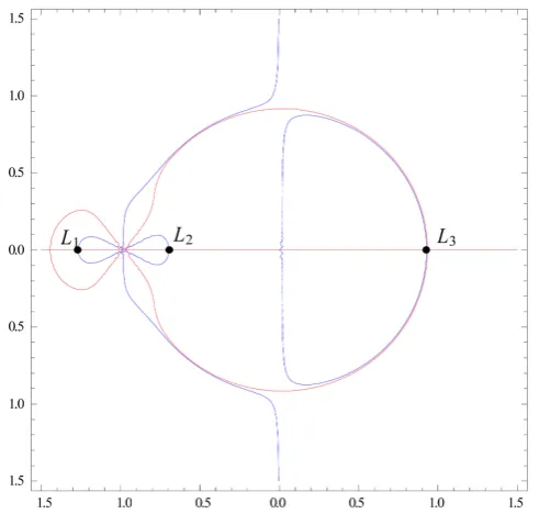
Figure 2. Locations of libration points for α=0,γ =1 (classical case).

[image:14.595.252.498.472.706.2]

DOI: 10.4236/ijaa.2019.91003 35 International Journal of Astronomy and Astrophysics In Figure 4, two collinear libration points L2 and L3 exist when

0.1, 0.98

α= γ = and σ1=0.01,σ2 =0.1, which contradicts theoretical

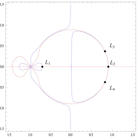
evolu-tion of the existence of the five libraevolu-tion points. In Figure 5, four coplanar points L L L2, 3, 4 and L5 exist for α=0.1,γ =0.96,σ1=0.1,σ2 =0.01 where

2

L and L3 are collinear and L4 and L5 are non-collinear which don’t form

the equilateral triangle with the primaries. The existence of L4 and L5 to the

[image:15.595.251.500.199.440.2]

right of the origin is a contradiction to the theoretical evolution of the existence of libration points in the classical case of Figure 2 (Theory of Orbits [11]).

Figure 4. Locations of libration points for α=0.1, =γ 0.98 (perturbed case).

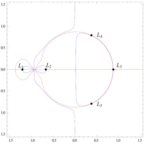
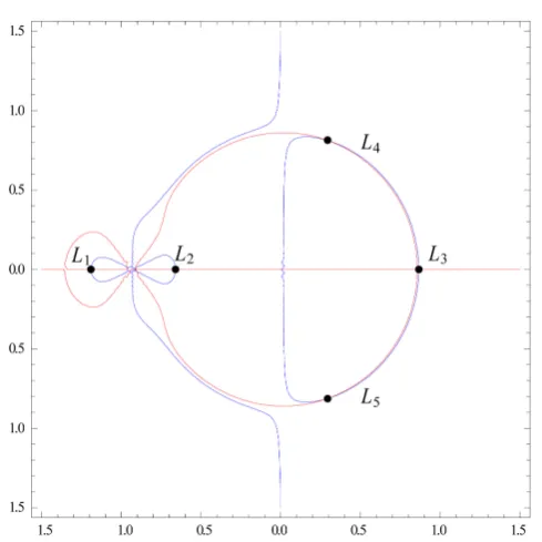
[image:15.595.256.497.468.707.2]

DOI: 10.4236/ijaa.2019.91003 36 International Journal of Astronomy and Astrophysics In Figure 6, when α =0.1,γ =0.94,σ1=0.1,σ2 =0.01, all the five libration

points exist with a difference. In Figure 6, the angular displacement of L4 and 5

L relative to L3 is more than that in Figure 5. Further when

γ

=0.92,

an-gular displacement of L4 and L5 relative to L3 is more in Figure 7 than that

in Figure 6 and similar case is repeated in Figure 8 for

γ

=0.9_{. Thus due to the}

variational parameters

α γ

, and triaxiality parameters σ1 and σ2, the location

[image:16.595.251.499.186.435.2]

of triangular libration points L4 and L5 has been shifted from left to right and

Figure 6. Locations of libration points for α=0.1, =γ 0.94 (perturbed case).

[image:16.595.250.501.461.709.2]

[image:17.595.252.497.62.307.2]

DOI: 10.4236/ijaa.2019.91003 37 International Journal of Astronomy and Astrophysics

Figure 8. Locations of libration points for α=0.1, =γ 0.9 (perturbed case). the angular distances of L4 and L5 relative to L3 increase with the decrease

of

γ

_{. From the above discussions, we conclude that for}

α

=0.1 _{and for} 0.94≤ ≤γ 0.9, all the five libration points exist with an increase in angular dis-placement of L4 and L5 relative to L3 with the decrease of

γ

and shifting of

4

L and L5 from positive to negative side of the x-axis.

Conflicts of Interest

The authors declare no conflicts of interest regarding the publication of this pa-per.

References

[1] Jeans, J.H. (1928) Astronomy & Cosmogomy. Cambridge University Press, Cam-bridge.

[2] Meshcherskii, L.V. (1949) Studies on the Mechanics of Bodies of Variable Mass. Gostekhizdat, Moscow.

[3] Shrivastava, A.K. and Ishwar, B. (1983) Equations of Motion of the Restricted Three-Body Problem with Variable Mass. Celestial Mechanics and Dynamical As-tronomy, 30, 323-328. https://doi.org/10.1007/BF01232197

[4] Singh, J. and Ishwar, B. (1985) Effect of Perturbations on the Stability of Triangular Points in the Restricted Three-Body Problem with Variable Mass. Celestial Me-chanics and Dynamical Astronomy, 35, 201-207.

https://doi.org/10.1007/BF01227652

[5] Das, R.K., Shrivastav, A.K. and Ishwar, B. (1988) Equations of Motion of Elliptic Restricted Three-Body Problem with Variable Mass. Celestial Mechanics and Dy-namical Astronomy, 45, 387-393. https://doi.org/10.1007/BF01245759

DOI: 10.4236/ijaa.2019.91003 38 International Journal of Astronomy and Astrophysics [7] El-Shaboury, S.M. (1990) Equations of Motion of Elliptically-Restricted Problem of a Body with Variable Mass and Two Triaxial Bodies. Astrophysics and Space Science, 174, 291-296.https://doi.org/10.1007/BF00642513

[8] Singh, J. (2008) Non-Linear Stability of Libration Points in the Restricted Three-Body Problem with Variable Mass. Astrophysics and Space Science, 314, 281-289.https://doi.org/10.1007/s10509-008-9768-9

[9] Hassan, M.R., Kumari, S. and Hassan, M.A. (2017) Existence of Libration Points in the R3BP with Variable Mass when the Smaller Is an Oblate Spheroid. International Journal of Astronomy and Astrophysics, 7, 45-61.

https://doi.org/10.4236/ijaa.2017.72005

[10] Volosov, V.M. (1972) Introductory Mathematics for Engineers. Mir Publishers, Moscow.