Estimating GARCH Modeling Using Metropolis Hastings Method in R

(1)

ISSN Print: 2161-718X

DOI: 10.4236/ojs.2018.86062 Dec. 20, 2018 931 Open Journal of Statistics

Estimating GARCH Modeling Using

Metropolis-Hastings Method in R

Min Wang

1,2

_{, Yunshun Wu}

1*

1_{School of Mathematical Sciences, Guizhou Normal University, Guiyang, China} 2_{School of Mathematical Sciences, Xiamen University, Xiamen, China}

Abstract

This paper mainly talks about a popular approach of volatility of a GARCH-type model in R, while the disturbances are independent and have identical Student-t distribution. It uses the Metropolis-Hastings method to perform the computations and gives the programs in details in R.

Keywords

Student’s t Distribution, Degree of Freedom, GARCH t Model, R, Metropolis-Hastings Method

1. Introduction

The R-project is an open statistics programming software. Modelling and fore-casting volatility or, in other word, the covariance structure of asset returns, is important. A central property of economic time series, being common to many financial time series, is that their volatility varies over time. Describing the vola-tility of an asset is a key issue in financial economics. Returns were modelled as independent and identically distributed over time. The most popular class of models for time-varying volatility is represented by GARCH type models [1]. GARCH models are commonly used for describing, estimating and predicting the dynamics of financial returns. Recent surveys of the existing GARCH models literature can be found in Davidson [2] and Rombouts et al. [3]. In contrast to Engle’s [4] ARCH model, a double autoregressive (DAR) model, which is a spe-cial case of the ARMA-ARCH models in Weiss [5] and an example of weak ARMA models in Francq and Zakoïan [6] [7], is also increasingly concerned about researchers. Under the assumption of the disturbance following a normal distribution, Ling [8] considered the structure and the maximum likelihood

es-How to cite this paper: Wang, M. and Wu, Y.S. (2018) Estimating GARCH Mod-eling Using Metropolis-Hastings Method in R. Open Journal of Statistics, 8, 931-938.

https://doi.org/10.4236/ojs.2018.86062

Received: November 23, 2018 Accepted:December 17, 2018 Published: December 20, 2018

http://creativecommons.org/licenses/by/4.0/

(2)

DOI:10.4236/ojs.2018.86062 932 Open Journal of Statistics

timation. In addition, stochastic volatility (SV) models have enjoyed great popu-larity in analyzing financial data in the last couple of decades [9].

In this paper, an R package named bayesGARCH [10] was mentioned to con-trast with our procedure. This package makes use of the priors based on the work of Nakatsuma [11], consists of Metropolis-Hastings (MH) algorithm [12] a proper algorithm to sample the posterior distribution.

The remainder of this paper is organized as follows. In Section 2 we describe the GARCH (1, 1)-t process and introduce how to estimate the parameters by using the Metropolis-Hastings method. Through an example, we contrast our model with the bayesGARCH package in Section 3. Section 4 provides the R procedure to execute our model in details. An empirical example is reported in Section 5, and Section 6 concludes this paper.

2. Univariate GARCH-t Model

Let Yt denote a asset return. The general structure of an asset return series modeled by a GARCH-type models can be written as Audronė Virbickaitė et al. 2014 [13]:

. t t t t t t Y =µ +a =µ +h_

In general  is a Normal variable. Without loss information, we set µ =t 0.

To capture the fat tail so prominent a Student-t distribution is used for condi-tional density. The model is, GARCH-t, is

(

2

)

2 2 2

1 0 1 1 1

| 0, , .

t t t t t t t

Y F− Sψ h h =α +αY− +βh− (1)

where

(

_0, 2

)

t t

S_ψ h is a Student-t distribution with mean 0 and ψ is the degree of freedom parameter. ht is the conditional variance given Ft−1 in the

GARCH (1, 1) model. α >0 0, α β ≥1, 0 are restrictions for positive variance,

and α β+ <1_{for the covariance stationarity. Then the posterior density}

func-tion could be:

(

)

(

)

(

)

(

)

( ) 1 ₁ 2 1 2 2 ₂

1 1 2

2

1 ₁

2

| 2 1 .

2 1

2

t

t t t

t y

f y h

h ψ ψ ψ ψ π ψ − + − −  

Γ_ + _ _ _

 _{ } _

= ⋅_ − _ ⋅ + 

−

   

Γ  _ _

F

(2)

It is indicated that the  obey the Student-t distribution in (1). The follow-ing, we will show how we get (2), the density distribution of  is

( )

₁

2 2 1 2 1 2 t p _ψ ψ ψ ψ π ψ + +  

Γ_ _ =

 

⋅ ⋅Γ_{ }_ + _

  



Through the equation Y ht = ⋅t t, the distribution of Yt is

(

)

(

)

(

1

)

(

1

)

t

t t t t t t t t t t

P Y _≤y ₌P h_{⋅ ≤}y ₌P _≤h y− ₌F h y− 

 

(3)

DOI: 10.4236/ojs.2018.86062 933 Open Journal of Statistics

( )

(

)

(

)

1 1 1

1 2 2 1

1

1 2 2 ₂

1 2 1 2 1 2 1 2 ₁ 2 t t

Y t t t t t

t t

t

p y p h y h h

h y

h y _h

ψ ψ ψ ψ ψ π ψ ψ ψ ψ ψ π − − − + − + − − − ₋ +  

Γ_ _

= ⋅ = ⋅

 

  

⋅ ⋅Γ_{ } + _

 _ _

+

 

Γ  _ _

  = ⋅ _ + _ ⋅   _ _ ⋅Γ     (3)

Because,Var

( )

t ₂ ψ ψ =

−

 , to ensure the conditional variance of Yt to be ht2,

we replace “ht” with “ 2 ht ψ

ψ − _⋅

”, then the (3) changed into (2).

Given a dataset Yt =

(

y y1, , ,2  yT

)

, model parameter Γ = Γ

(

α α β ψ0, , ,1

)

and the posterior density is

(

)

( )

(

1

)

1

| T T t| t

t

p Y p f y −

=

Γ ∝ Γ ⋅

_∏

F

According to Jensen [14], the priors are independent and identically distri-buted (IID) as N (0, 100) with the following restrictions α >0 0, α ≥1 0,β ≥0

to impose identification and ψ >2_{. Since the variance is non-negative, the}

pos-itive constraints on coefficients are reasonable. The restriction on the degrees of freedom parameter ψ _{ensures the conditional variance to be finite and the} re-strictions on the GARCH parameters α0, α1 and β guarantee its positivity.

One of the most popular MCMC algorithm used in estimating GARCH model parameters, is the Metropolis-Hastings (MH) method. We emphasize the fact that only positivity constraints are implemented in the MH algorithm; no sta-tionarity conditions are imposed in the simulation procedure. We employ a MH sampler. Given the current value Γ of the chain, the proposal Γ′_{is sampled} from

( )

(

₍

,

)

₎

with probability

,100 with probability 1

N V p

h

N V p

 Γ  ′ Γ _ Γ −  

where V is the inverse Hessian matrix of log

(

p

(

Γ|YT

)

. The accepted probability

equal to min

(

₍

|

)

₎

,1 | T T p Y p Y        

 , and p=0.9 empirically. After the test sample col-lecting the new

{ }

( )

1

N i

i=

Γ , the predictive density is

(

)

(

( ) ( )

)

1 1 1

1

| N | 0, i , i .

t t t t

i

p y Y f y h

N ψ

+ + +

=

≈

∑

3. The Priors and bayesGARCH Package

(4)

GRACH model, then we’ll describe the difference of the priors between our model and the package. The package bayesGARCH provides functions for the Bayesian estimation of the parsimonious and effective GARCH (1, 1) model with Student-t innovations. The priors in the bayesGARCH package distributions on

0

α _{is a bivariate truncated Normal distribution;}α₁_{is a univariate truncated} Normal distribution; β_{is a translated Exponential distribution. The} estima-tion procedure is fully automatic and thus avoids the tedious task of tuning an MCMC sampling algorithm. It is obviously there are some differences set of priors between our model and the package, so we couldn’t cite the package di-rectly. Next, we will show the estimation results to demonstration that the dif-ferent priors could inference the estimation result.

3.1. Example

We set the initial value of Γ is (1, 0.2, 0.4, 5). 800 simulation values are ob-tained by simulation in R.

800

R T> =

( (0, ))

R y c rep T> =

[1] 0.5; [1] 0.5

R y> = h =

0 1; 1 0.2; 0.4; 5

R alpha> = alpha = beta= psi=

( 2 : )

R for iin T>

{

+

2

[ ] 0 1 [ 1] [ 1]

h i alpha alpha y i beta h i

+ = + ∗ − + ∗ −

[ ] (1, )

y i rt psi

+ =

[ ] ( [ ]) [ ]

y i sqrt h i y i

+ = ∗

}

+

Then we use bayesGARCH package to estimate Γ, we remain the number of MCMC chains and the length of each MCMC chain to be the default value.

( )

MCMC< −bayesGARCH y

( , . 50)

smpl< −formSmpl MCMC l bi=

( )

summary smpl

We receive the estimation of Γ is (1.2630, 0.2367, 0.4829, 11.3285). Obviously, there’s a big difference estimation of ψ _{and the estimation of other parameters} is equally unsatisfactory.

3.2. The Priors

(5)

[image:5.595.206.529.90.181.2]

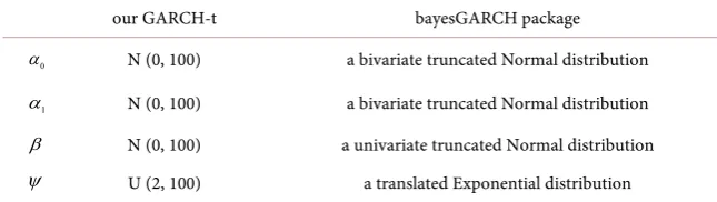
DOI: 10.4236/ojs.2018.86062 935 Open Journal of Statistics Table 1. The difference sets of priors.

our GARCH-t bayesGARCH package

0

α _{N (0, 100)} _{a bivariate truncated Normal distribution}

1

α N (0, 100) a bivariate truncated Normal distribution

β _{N (0, 100)} _{a univariate truncated Normal distribution}

ψ _{U (2, 100)} _{a translated Exponential distribution}

Note. This table shows the priors set in our model are all independent each other and more typical.

4. Conducting GARCH-t in R

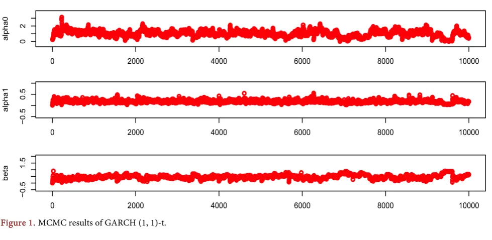
The estimate results in our model

In this section, we design and developed the R program. We will show the whole procedure of how we conduct GARCH-t in R. Our results is (1.0103, 0.1838, 0.4694, 9.2587) is closer to the true value, and we can see the procedure in Figure 1.

The R program

We set the all necessary initial values to be zero, the number of MCMC chain to be 10,000, meanwhile Γ is a 10,000 times 4 matrix. We leave out the R programs for these simple settings, giving only the necessary parts of the program.

( 2 : )

R for i in> N

{

R>

(1,0,1)

R u runif> =

(1, [ 1,1],0.1 ) ( 0.9)

R gammaA rnorm gamma i> = − ∗ ∗ <=v u

(1, [ 1,1],5 ) ( 0.9)

rnorm gamma i v u

+ − ∗ ∗ >

( 2 : )

R for j in T>

{

R>

2 2 2 2

[ ] [ 1,2] [ 1] [ 1,3] [ 1]

R hh j> =gammaA +gamma i− ∗y j− +gamma i− ∗hh j−

2 2 2

2

[ ] [ 1,1] [ 1,2] [ 1]

[ 1,3] [ 1]

R oldhh j gamma i gamma i y j

gamma i oldhh j

> = − + − ∗ −

+ − ∗ −

( / ( ), [ 1,4]) / ( )

R prop dt y sqrt hh gamma i> = − sqrt hh

/ ( ) ( ), () .

where y sqrt hh tψ and dt returns the density value of the t distribution

( / ( ), [ 1,4]) / ( )

R old dt y sqrt oldhh gamma i> = − sqrt oldhh

( ( ) ( ))

R ratio sum log prop log old> = −

( )

R ratio exp ratio> =

[ ,1] [ 1,1] ( [ 1,1])*( (1) )

R gamma i> =gamma i− + gammaA gamma i− − runif <ratio

The above procedure could give the estimate value of α0, and the estimation

(6)

5. Empirical Application

[image:6.595.56.546.169.408.2]

This section will use Metropolis-Hastings method by the actual financial data to fit the model. The using data is the DAX(Ibis) index of German in European stock market, a total of 1860 data. In order to make the data smooth, we need to do some processing to the original data. Let xt denote the logarithm and yt denote the order difference of xt, i.e. yt = −x xt t−1, see Figure 2.

Figure 1. MCMC results of GARCH (1, 1)-t.

[image:6.595.57.543.299.682.2]

(7)

DOI: 10.4236/ojs.2018.86062 937 Open Journal of Statistics

We apply the R program in the section 5 to estimate the DAX data, achieve the result of Γ is (0.0028, 0.0600, 0.0676, 7.7485). That is, the equation of

va-riance is 2 2 2

1 1

0.0028 0.0600 0.676

t t t

h = + ∗Y− + ∗h− . Through compute the

Ljung-Box test statistic for examining the null hypothesis of independence in ARCH model, we get the χ squared 0.0023 with p-value 0.9621. It obvious to show our GARCH (1, 1)-t model is sufficient.

6. Conclusion

In this article, the R program to estimate GARCH-t model has been developed. The parameters’ distribution has been modeled using Gaussian model with the most common setting. The results we achieved in each of our experiments with either simulation study or real data application, are quite encouraging.

Foundation

This research was partially supported by the PhD research startup foundation of Guizhou Normal University (Grant No. GZNUD[2017]27) & Science and Technology Foundation of Guizhou Province (LKS[2013]5 & LKS[2012]11), China. & Teaching Project of Guizhou Normal University in 2016: Contract No. [2016] XJ No. 09.

Conflicts of Interest

The authors declare no conflicts of interest regarding the publication of this pa-per.

References

[1] Bollerslev, T. (1986) Generalized Autoregressive Conditional Heteroscedasticity. Journal of Econometrics, 31, 307-327.

https://doi.org/10.1016/0304-4076(86)90063-1

[2] Davidson, J. (2012) Moment and Memory Properties of Linear Conditional Hete-roscedasticity Models, and a New Model. Journal of Business & Economic Statistics, 22, 16-29.https://doi.org/10.1198/073500103288619359

[3] Rombouts, J., Stentoft, L. and Violante, F. (2014) The Value of Multivariate Model Sophistication: An Application to Pricing Dow Jones Industrial Average Options. International Journal of Forecasting, 30, 78-98.

https://doi.org/10.1016/j.ijforecast.2013.07.006

[4] Engle, R.F. (1982) Autoregressive Conditional Heteroscedasticity with Estimates of the Variance of U.K. Inflation. Econometrica, 50, 987-1007.

https://doi.org/10.2307/1912773

[5] Weiss, A.A. (1986) Asymptotic Theory for ARCH Models: Estimation and Testing. Econometric Theory, 2, 107-131.https://doi.org/10.1017/S0266466600011397 [6] Francq, C. and Zakoïan, J.M. (1998) Estimating Linear Representations of

Nonli-near Processes. Journal of Statistical Planning & Inference, 68, 145-165. https://doi.org/10.1016/S0378-3758(97)00139-0

(8)

I—Mathematics, 83, 369-394.https://doi.org/10.1016/S0378-3758(99)00109-3 [8] Ling, S. (2007) A Double AR(p) Model: Structure and Estimation. Statistica Sinica,

17, 161-175.

[9] Jacquier, E., Polson, N.G. and Rossi, P. (2004) Bayesian Analysis of Stochastic Vola-tility Models with Fat-Tails and Correlated Errors. Journal of Econometrics, 122, 185-212.https://doi.org/10.1016/j.jeconom.2003.09.001

[10] Ardia, D. (2007) bayesGARCH: Bayesian Estimation of the GARCH(1,1) Model with Student-t Innovations in R.

http://CRAN.R-project.org/package=bayesGARCH

[11] Nakatsuma, T. (1998) A Markov-Chain Sampling Algorithm for GARCH Models. Studies in Nonlinear Dynamics & Econometrics, 3, 107-117.

https://doi.org/10.2202/1558-3708.1043

[12] Chin, S. and Greenberg, E. (1995) Markov Chain Monte Carlo Simulation Methods in Econometrics. Econometrics, 12, 409-431.

[13] Virbickaitė, A., Ausín, M.C. and Galeano, P. (2015) A Bayesian Non-Parametric Approach to Asymmetric Dynamic Conditional Correlation Model with Applica-tion to Portfolio SelecApplica-tion. Computational Statistics and Data Analysis, 100, 814-829.https://doi.org/10.1016/j.csda.2014.12.005

[14] Jensen, M.J. and Maheub, J.M. (2013) Bayesian Semiparametric Multivariate GARCH Modeling. Journal of Econometrics, 176, 3-17.

https://doi.org/10.1016/j.jeconom.2013.03.009

[15] Geweke, J. (1993) Bayesian Treatment of the Independent Student-t Linear Model. Journal of Applied Econometrics, 8, S19-S40.