A New Method for the Exact Solution of Duffing Equation

(1)

ISSN Online: 2327-4379 ISSN Print: 2327-4352

DOI: 10.4236/jamp.2018.612225 Dec. 31, 2018 2718 Journal of Applied Mathematics and Physics

A New Method for the Exact Solution of Duffing

Equation

Ossou Nazila Fred Nelson

1

, Zheng Yu

2

, Bambi Prince Dorian

1

, Yuya Wang

1

1_{College of Economics, Shanghai University, Shanghai, China}

2_{School of Economics & Management, Tongji University, Shanghai, China}

Abstract

A lot of methods, such as Jacobian elliptic function analysis, are used to look for the explicit exact solution of Duffing differential equation. The key of the analysis is to construct quotient trigonometric function, and then nonlinear algebraic equation set theory and method are used for the solution of some kinds of nonlinear Duffing differential equation. In this paper, the exact solu-tion of Duffing equasolu-tion is obtained by using constant variasolu-tion method, making use of the formula to solve cubic equations and general solution of the homogeneous equation of Duffing equation with appropriate Constant m and function f t( ).

Keywords

Duffing Equation, Exact Solution, Constant Variation Method

1. Introduction

The Duffing equation is a non-linear second-order differential equation. The equation describes the motion of a damped oscillator with a more complicated potential than in simple harmonic motion; in physical terms, it models, for ex-ample, a spring pendulum whose spring’s stiffness does not exactly obey Hooke’s law. It is also an example of a dynamical system that exhibits chaotic behavior.

Many of the dynamic behavior of mechanical power model can be described by a single degree of freedom oscillator [1] [2] [3] [4] [5]. The systems can be described by the following equation

( ) ( , , )

x f x= +εg x x t x R∈

 

Alex (2013) discussed the exact solution of a cubic-quintic Duffing oscillator of the form [6]

How to cite this paper: Nelson, O.N.F., Yu, Z., Dorian, B.P. and Wang, Y.Y. (2018) A New Method for the Exact Solution of

Duffing Equation. Journal of Applied

Ma-thematics and Physics, 6, 2718-2726.

https://doi.org/10.4236/jamp.2018.612225

(2)

DOI: 10.4236/jamp.2018.612225 2719 Journal of Applied Mathematics and Physics

3 5 ₀

x Ax Bx Gx+ + + = 

Alex’s idea is both simple and enlightening, he turn looking for exact solution into solving algebraic equations set. Without lose of generally, in this paper, we consider the following Duffing equation without external force and damping

3 ₀

x x x− + =

 (1.1) Talay’s solve approach is much complex. He assumes that the Equation (1.1) has boundary conditions in the form

(0) 0

x = and x(±∞ =) 0

Given x(0)=a_, x t( )=ay t( ), where a is an undetermined parameter, the Equation (1.1) becomes

2 3 ₀

y y a y− + =

 (1.2)

Equation (1.2) satisfies the following boundary conditions (0) 1

y = _, y(0) 0= , y( ) 0±∞ = _(1.3) Additionally, Talay assumed that the solution of Equation (1.2) can be ex-pressed by index Series in the form

0 1

( ) mt ( ) ( )

m k

k

y t c e− y t ∞ y t

=

∑

= +

∑

According to the boundary conditions, he deduces

2 0( ) 2 t t

y t ₌ e− ₋e−

2 3 4 5 6

1 0 1 2

2 3 4 5 6

4 1 1

( ) [ ( )]

5 4 35

5 35 7 35 1

( )

64 36 4 64 16

t t t t t t t

t t t t t t

y t e e e e e c e c e

e e e e e e

γ

− − − − − −

= + − + − + +

= − + − + −



In the last few years, many scientists work hard to look for exact solutions and to develop some efficient procedures. However, what the key of problem is, the different type of nonlinear differential equation can only be efficiently solved by different corresponding methods. For instant, the Jacobi elliptic function expan-sion method [7], the exp-function method [8], the F-expanexpan-sion method [9], the tanh method [10], the auxiliary equation method [11], the simplest equation method [12], and linearized harmonic balance method [13] are reliable methods for obtaining exact solutions of specific types of nonlinear differential equations.

(3)

DOI: 10.4236/jamp.2018.612225 2720 Journal of Applied Mathematics and Physics a method for obtaining exact solutions for Duffing and double-well Duffing eq-uations [16]. What he used is traditional quotient trigonometric function expan-sion method, and his solution procedure is similar to the exp-function method. However, his result in third section has a distance to reach perfect.

Exact analytical solutions for a family of autonomous ordinary differential equations arising in connection with many important applied problems such as a cubic-quintic Duffing oscillator, Helmholtz–Duffing oscillator, and nonlinear Schrödinger equation are considered. Recently, some theory and applications are found in many contexts, such as, Jiang et al. (2012) presented a new approach via the well-known Poincaré-Birkhoff theorem to obtain the existence of period-ic solutions to impulsive problems, they considered an impulsive Duffing equa-tion, and then found the possibility of applying a generalized form of the Poin-caré-Birkhoff theorem due to Ding to construct infinitely many periodic solu-tions of the impulsive Duffing equation even in a resonance case [17]. Jaume and Ana (2015) studied the periodic solutions of a kind of non-autonomous Duffing differential equation with forced pendulum. And, they obtained the condition for that the non-autonomous Duffing differential system has a periodic solution such that it tends to the periodic solution when forced pendulum satisfied with some conditions [18]. Gholam and Emmanuel (2015) have provided a set of in-equalities that helps in finding transformation to obtain solutions to other Duff-ing equations from a known set of solutions to a related equation in a systematic manner [19]. Alexander (2018) has obtained the sufficient and necessary condi-tions for the existence of a positive periodic solution to a kind of non-autonomous Duffing type equation [20]. David and Douglas (2018) perform a complete anal-ysis of the effect on the asymptotic dynamics of the insertion of delays into a sort of unforced Duffing type equation [21].

One of the most exciting recent advances of nonlinear science has been the development of some methods to look for exact solutions of nonlinear differen-tial equations. It is important that many mathematical models are described by nonlinear differential equations and exact solutions are preferable instead of ap-proximate ones. The aim of this paper is to put forward constant variation me-thod to derive the exact solution of a Duffing equation of the form (1.1). The exact solution of Duffing equation is obtained by solving cubic equations and looking for appropriate constant m and function f t( ).

2. Constant Variation Method

In general, the Duffing equation does not admit an exact symbolic solution. However, many approximate methods work well:

 Expansion in a Fourier series will provide an equation of motion to arbitrary precision.

 The cubic term also called the Duffing term can be approximated as small and the system treated as a perturbed simple harmonic oscillator.

(4)

 Any of the various numeric methods such as Euler’s method and Runge-Kutta can be used.

In the special case of the undamped and unforced, an exact solution of Duff-ing equation has been obtained usDuff-ing our constant variation method

Now, let’s begin at the solution of the homogeneous linear equations. The homogeneous linear equations corresponding to Equation (1.1) is

0

x x− =

 (2.1) Its general solution is

1 t 2 t

x c e c e₌ ₊ − _(2.2)

Assume we have functions c t1( ) and c t2( ), such that the solution of

Equa-tion (1.1) has the form as

1( ) t 2( ) t

x c t e c t e₌ ₊ − _(2.3)

Taking Equation (2.3) into Equation (1.1), we obtain following differential equation

3 1( ) t 2( ) t 2( ( )1 t 2( ) ) ( ( )t 1 t 2( ) )t 0

c t e c t e₊ − ₊ c t e c t e₋ − ₊ c t e c t e₊ − ₌

    (2.4)

Because functions c t1( ) and c t2( ) are discretionary, hence, we let

1( ) 2( ) ( )

c t =c t =c t .

Then, Equation (2.4) becomes

3 3

( )( t t) 2 ( )( t t) ( )( t t) 0

c t e e_ ₊ − ₊ c t e e_ ₋ − ₊c t e e₊ − ₌ _(2.5)

Therefore, we obtain a more compact differential equation form for unknown function c t( ) .

If we can find an undetermined constant m and an undetermined function ( )

f t , such that they satisfy with following equation

3 2

( ) ( ) ( )( t t)

f t ₌mc t c t e e₋ ₊ − _(2.6)

Then, it is possible for us to reduce solving differential Equation (2.5) to looking for a couple of undetermined constant m and undetermined function

( )

f t . Our main conclusions as follows.

Theorem 1. The Equation (2.5) has solutions if only and if the following equ-ations set have solutions for given constant m and undetermined function f t( ).

{

3 2

( ) 2 ( ) ( ) ( )

( )( ) ( ) ( ) 0

t t

e e

c t c t mc t f t

e e

c t e e mc t f t

−

 −

+ + =



+ 

 ₊ ₋ ₊ ₌



  _(2.7)

Proof: Let _{z c t e e}₌ ( )( t₊ −t)_{, then Equation (2.6) leads to a cubic equation as}

3 _{( )(} t t_{) 0}

z mz f t e e₋ ₊ ₊ − ₌ _(2.8)

Its solutions can be expressed as

3 2

3

2 2

3

4

( )( ) ( )( )

27 2

4

( )( ) ( )( )

27 2

t t t t

m

f t e e f t e e

z

m

f t e e f t e e

− −

− + + + −

=

− + − + −

+

(5)

DOI: 10.4236/jamp.2018.612225 2722 Journal of Applied Mathematics and Physics Specially, if m=0_{, we have the simplest representation as follows}

3 _{( )(} t t₎

z_{= −} f t e e₊ − _.

Notice that Equation (2.7) has denominators in the form as (_{e e}t₊ −t)_{,so let} 3

4

( )

( t t)

k f t

e e−

− =

+ (2.10)

Applying function (2.10) to equations set (2.7), we get _k3 ₌₈_k_{, it means}

2 2

k= _or k =0_.

On the other hand, we can prove that _k3_{is forever equal to 8}_k_when _m₌₀_.

Actually, if m=0, then ( ) ₍ t 3t₎4

k f t

e e−

− =

+ , meanwhile, we have

( t t)

k z

e e−

= +

Let’s make a transformation: _{z c t e e}₌ ( )( t₊ −t)_{, then}

2

( )

( t t)

k c t

e e−

= +

Applying c t( ) and its first derivative and second derivative to equations set (2.7), we have

2 2 3

4 3 4

( ) 3( )

2 4

( ) ( ) ( )

t t t t t t t t

e e e e e e e e k

k k

e e e e e e e e

− − − −

+ − − − −

+ ⋅ =

+ + + + (2.11)

Equation (2.11) follows _k3₌₈_k _{immediately. This finishes the proof of}

theorem1.

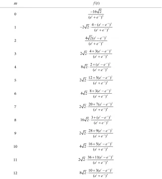
We have showed a few representative integer parameters m and functions in Table 1.

In fact, m is not only integer, but it maybe any fractional as well. Some values of m and respective function are showed in Table 2.

3. Applications

In this section, we shall give some examples to explain our constant variation method.

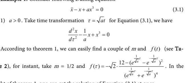
Example 1. Consider following Duffing equation

3 ₀

x x ax− + =

 (3.1) 1) a>0. Take time transformation τ = at for Equation (3.1), we have

2

3 2

1 ₀

d x _{x x} a

d

τ

− + =

According to theorem 1, we can easily find a couple of m and f t( ) (see

Ta-ble 2), for instant, take m = 1/2 and

1 1

2

1 1

4

12 ( )

( ) 2

( )

a a

e e

f

e e

τ τ

τ

−

− −

= − ⋅

+

. In the

[image:5.595.216.541.569.716.2]

(6)

[image:6.595.210.539.92.456.2]

DOI: 10.4236/jamp.2018.612225 2723 Journal of Applied Mathematics and Physics Table 1. Integer parameter m and function f t( ).

m f t( )

0 4

16 2 (_{e e}t −t)

− +

1 42

4 ( )

2 2 ( ) t t t t e e e e − − − − − ⋅ +

2 4 2

4 2( )

( ) t t t t e e e e − − − +

3 4 2

4 3( ) 2 2 ( ) t t t t e e e e − − + − ⋅ +

4 42

2 ( )

8 2 ( ) t t t t e e e e − − + − ⋅ +

5 4 2

12 5( ) 2 2 ( ) t t t t e e e e − − + − ⋅ +

6 4 2

8 3( ) 4 2 ( ) t t t t e e e e − − + − ⋅ +

7 4 2

20 7( ) 2 2 ( ) t t t t e e e e − − + − ⋅ +

8 42

3 ( )

16 2 ( ) t t t t e e e e − − + − ⋅ +

9 4 2

28 9( ) 2 2 ( ) t t t t e e e e − − + − ⋅ +

10 4 2

16 5( ) 4 2 ( ) t t t t e e e e − − + − ⋅ +

11 4 2

36 11( ) 2 2 ( ) t t t t e e e e − − + − ⋅ +

12 4 2

10 3( ) 8 2 ( ) t t t t e e e e − − + − ⋅ +

Table 2. Fractional parameter m and function f t( ).

m f t( )

1 2

2 4 12 ( ) 2 ( ) t t t t e e e e − − − − − ⋅ + 1 3 2 4

2 2 20 ( )

3 ( )

t t t t e e e e − − − − − ⋅ + 1 4 2 4

2 2 14 ( )

2 ( )

t t t t e e e e − − − − − ⋅ + 1 5 2 4

2 2 36 ( )

5 ( )

t t t t e e e e − − − − − ⋅ + 1 6 2 4

2 44 ( )

3 ( )

t t t t e e e e − − − − − ⋅ + 1 7 2 4

2 2 52 ( )

7 ( )

t t t t e e e e − − − − − ⋅ + 1 8 2 4

2 60 ( )

4 ( )

t t t t e e e e − − − − − ⋅ + 1 9 2 4

2 2 68 ( )

9 ( )

[image:6.595.205.538.491.739.2]

(7)

2 2 _{2 2 ,} ₀

cosh cosh

x a

a t

a

τ

= = > _(3.2)

2) a<0. Take time transformation τ = −at _{for Equation (3.1), in same}

way we also get

2 2 _, ₀

sinh

x a

a t

= <

− (3.3)

Example 2. Vasile (2011) discussed the unforced and undamped double-well Duffing equation [16]

2 3

0 0

x−

ω

x+

β

x =

 (3.4) where β_{is a positive constant which may not be a small value.}

We can easily obtain exact solution of Equation (3.4) in the same way as ex-ample 1.

0

2 2 cosh( )

x

t

β

ω

= _(3.5)

Example 3. Jaume and Ana (2013; 2015) discussed following modified Duff-ing differential equation [15] [19]

3 _{( , )}

y ay+ −

ε

y =

ε

h y y

  (3.6)

In the special case h=0,a<0_{, we obtain one of the solutions of Equation} (3.6) at once in the same way as example1.

2 2 _, ₀

cosh( )

y

at

ε

= <

− − (3.7)

2 2 _, ₀

sinh( )

y

at

ε

= >

− (3.8)

Example 4. By using Jacobian elliptic function, Alex (2013) derive the exact solution of a cubic-quintic Duffing oscillator of the form [14]

3 5 ₀

x Ax Bx Gx+ + + =

 (3.9)

Let’s discuss the special case G=0,A<0,B>0_{. Take time transformation} ( 0)

Bt B

τ

= > _{for Equation (3.9), then (3.9) can be turned into}

2

3

2 0

d x A x x B

d

τ

+ + =

According the result in example 3, one can get the solution at once

2 2 _, ₀

cosh( )

x B

B At

= >

− and

2 2 _, ₀

sinh( )

x B

B At

= <

− − (3.10)

Acknowledgements

(8)

DOI: 10.4236/jamp.2018.612225 2725 Journal of Applied Mathematics and Physics (71171128) and Shanghai University’s horizontal project (Project name: compa-ny convertible bond pricing method and its application).

Conflicts of Interest

The authors declare no conflicts of interest regarding the publication of this pa-per.

References

[1] Ho, C. and Lang, Z.-Q. (2014) Stephen A. Billings. A Frequency Domain Analysis of the Effects of Nonlinear Damping on the Duffing Equation. Mechanical Systems and Signal Processing, 45, 49-67. https://doi.org/10.1016/j.ymssp.2013.10.027 [2] Cveticanin, L. (2001) Analytic Approach for the Solution of the Complex-Valued

Strong Non-Linear Differential Equation of Duffing Type. Physica A, 297, 348-360.

https://doi.org/10.1016/S0378-4371(01)00228-X

[3] Du, L.-C. and Mei, D.-C. (2011) Stochastic Resonance, Reverse-Resonance and sto-chastic Multi-Resonance in an Underdamped Quartic Double-Well Potential with Noise and Delay. Physica A, 390, 3262-3266.

https://doi.org/10.1016/j.physa.2011.05.006

[4] Cveticanin, L. (2003) Analytic Solution of the System of Two-Coupled Differential Equations with the Fifth-Order Non-Linearity. Physica A, 317, 83-94.

https://doi.org/10.1016/S0378-4371(02)01323-7

[5] Mallick, K. and Marcq, P. (2003) Effects of Parametric Noise on a Nonlinear Oscil-lator. Physica A, 325, 213-219. https://doi.org/10.1016/S0378-4371(03)00200-0 [6] Elías-Zúñiga, A. (2013) Exact Solution of the Cubic-Quintic Duffing Oscillator.

Ap-plied Mathematical Modelling, 37, 2574-2579.

https://doi.org/10.1016/j.apm.2012.04.005

[7] Liu, S.K., Fu, Z.T., Liu, S.D. and Zhao, Q. (2001) Jacobi Elliptic Expansion Method and Periodic Wave Solutions of Nonlinear Wave Equations. Physics Letters A, 289, 69-74. https://doi.org/10.1016/S0375-9601(01)00580-1

[8] Dai, C.Q. and Zhang, J.F. (2009) Application of He’s Exp-Function Method to the Stochastic mKdV Equation. Int. J. Nonlinear Sci. Num., 10, 675-680.

[9] Elhanbaly, A. and Abdou, M. (2007) Exact Travelling Wave Solutions for Two Non-linear Evolution Equations Using the Improved F-Expansion Method. Math. Com-put. Modelling, 46, 1265-1276. https://doi.org/10.1016/j.mcm.2007.01.004

[10] Ugurlu, Y. and Kaya, D. (2008) Exact and Numerical Solutions of Generalized Drinfeld-Sokolov Equations. Phys. Lett. A, 372, 2867-2873.

https://doi.org/10.1016/j.physleta.2008.01.003

[11] Sirendaoreji. (2004) New Exact Traveling Wave Solutions for the Kawahara and Modified Kawahara Equation. Chaos Solitons Fractals, 19, 147-150.

https://doi.org/10.1016/S0960-0779(03)00102-4

[12] Vitanov, N.K. (2010) Application of Simplest Equations of Bernoulli and Riccati Kind for Obtaining Exact Travelling-Wave Solutions for a Class of PDEs with Po-lynomial Nonlinearity. Commun. Nonlinear Sci Numer. Simul., 15, 2050-2060.

https://doi.org/10.1016/j.cnsns.2009.08.011

(9)

Os-DOI: 10.4236/jamp.2018.612225 2726 Journal of Applied Mathematics and Physics cillators. International Journal of Non-Linear Mechanics, 43, 993-999.

https://doi.org/10.1016/j.ijnonlinmec.2008.05.001

[14] Li, K.Q., Wang, S.J. and Zhao, Y.G. (2013) Multiple Periodic Solutions for Asymp-totically Linear Duffing Equations with Resonance (II). Journal of Mathematical Analysis and Applications, 397, 156-160. https://doi.org/10.1016/j.apm.2012.04.005 [15] Llibre, J. and Rodrigues, A. (2013) A Note on the Periodic Orbits of a Kind of

Duff-ing Equations. Applied Mathematics and Computation, 219, 8358-8365.

https://doi.org/10.1016/j.amc.2012.11.087

[16] Marinca, V. and Herişanu, N. (2011) Explicit and Exact Solutions to Cubic Duffing and Double-Well Duffing Equations. Mathematical and Computer Modelling, 53, 604-609. https://doi.org/10.1016/j.mcm.2010.09.011

[17] Jiang, F.F., Shen, J.H. and Zeng, Y.T. (2012) Applications of the Poincaré-Birkhoff Theorem to Impulsive Duffing Equations at Resonance. Nonlinear Analysis: Real World Applications, 13, 1292-1305. https://doi.org/10.1016/j.nonrwa.2011.10.006

[18] Llibre, J. and Rodrigues, A. (2015) A Non-Autonomous Kind of Duffing Equation. Applied Mathematics and Computation, 251, 669-674.

https://doi.org/10.1016/j.amc.2014.11.007

[19] Zakeri, G.-A. and Yomba, E. (2015) Exact Solutions of a Generalized Autonomous Duffing-Type Equation. Applied Mathematical Modelling, 39, 4607-4616.

https://doi.org/10.1016/j.apm.2015.04.027

[20] Lomtatidze, A. and Šremr, J. (2018) On Periodic Solutions to Second-Order Duffing Type Equations. Nonlinear Analysis: Real World Applications, 40, 215-242.

https://doi.org/10.1016/j.nonrwa.2017.09.001

[21] Hill, D.C. and Shafer, D.S. (2018) Asymptotic and Stability of the Delayed Duffing Equation. J. Differential Equations, 265, 33-68.