warwick.ac.uk/lib-publications
A Thesis Submitted for the Degree of PhD at the University of Warwick
Permanent WRAP URL:
http://wrap.warwick.ac.uk/91306
Copyright and reuse:
This thesis is made available online and is protected by original copyright.
Please scroll down to view the document itself.
Please refer to the repository record for this item for information to help you to cite it.
Our policy information is available from the repository home page.
Michail Fasoulakis
A thesis submitted to the University of Warwick in partial fulfilment of the requirements
for the degree of Doctor of Philosophy
Department of Computer Science
Acknowledgements
At the end of this journey, I would like to thank some people. First of all, I
would like to thank two brilliant people, my supervisors Artur Czumaj and
Marcin Jurdzi´nski. Any step of improvement that I did as researcher and
as human being I owe that to them. Then, I would like to thank my
“aca-demic father”, Apostolos Traganitis, who showed me the route of research.
Also, I would like to thank Argyrios Deligkas, John Fearnley and Rahul
Savani for our excellent collaboration in the paper [13]. Especially, many
thanks to Argyrios Deligkas for our discussions on the Tsaknakis-Spirakis
algorithm. Many thanks to Martin Gairing and Matthias Englert for being
my examiners and for their valuable comments on the thesis. Furthermore, I
would like to thank the University of Warwick, the department of Computer
Science and the DIMAP research centre. I really feel lucky that I had the
opportunity to study in such an academic environment.
During the period in Warwick I was lucky to make many friends. Many
thanks to Adam, Alex, Andrzej, Angelos, Angelos, Chimere, Dario, Ebrahim,
Giorgos, James, Jan, Joao, Jun, Kostas, Lehilton, Lukas, Matthew, Nikos,
Nick, Peter, Rafael, Tasos and Theano. Sorry if I forget anyone.
Finally, I would like to thank my parents Evangelia and Ioannis, and my
sister Stella for being the “fixed point” of my life. I dedicate this thesis to
them.
Declarations
I have not submitted any work presented in this dissertation for any previous
degree, or a degree at another university. All the work has been conducted
during my period of study at the University of Warwick. The results
pre-sented in this dissertation have been a result of collaborative work with my
PhD supervisors Artur Czumaj and Marcin Jurdzi´nski, and I have made
major and fundamental contributions to all of them. Preliminary versions
of the work have been published or have been accepted for publication:
parts of the results in Chapter 2 and 3 have been accepted for publication
in AAMAS 2017 [14, 15], the results in Section 2.5 and in parts of the
In-troduction have been published in SAGT 2014 [16], the results in Chapter 4
have been published in IJCAI 2015 [17], and the results in Chapter 5 have
been published in AAMAS 2016 [18]. Some results presented in section 2.2
and Chapter 6 form a part of the paper published in WINE 2016 [13], which
is the result of collaborative work with Artur Czumaj, Argyrios Deligkas,
John Fearnley, Marcin Jurdzi´nski, and Rahul Savani.
Abstract
The problem of finding equilibria in non-cooperative games and
understand-ing their properties is a central problem in modern game theory. After John
Nash [45] proved that every finite game has at least one equilibrium
(so-called Nash equilibrium), the natural question arose whether we can
com-pute one efficiently. After several years of extensive research, we now know
that the problem of finding a Nash equilibrium is PPAD-complete even for two-player normal-form games [10] (see also [21]), making the task of
find-ing approximate Nash equilibria one of the central questions in the area
of equilibrium computation. In this thesis our main goal is a new study
of the complexity of various variants of the approximate Nash equilibrium.
Specifically, we study algorithms for additive approximate Nash equilibria
in bimatrix and multi-player games. Then, we study algorithms for
rela-tive approximate Nash equilibria in multi-player games. Furthermore, we
study algorithms for optimal approximate Nash equilibria in bimatrix games
and finally we study the communication complexity of additive approximate
Nash equilibria in bimatrix games.
Contents
1 Introduction 1
1.1 New contributions . . . 5
1.2 Definitions — bimatrix games . . . 6
1.3 Definitions — multiplayer games . . . 14
I Algorithms for approximate Nash equilibria 16 2 Additive approximate Nash equilibria 18 2.1 Tsaknakis-Spirakis algorithm . . . 19
2.1.1 Directional Derivative of Regret . . . 19
2.1.2 An LP for Minimizing Directional Derivative . . . 25
2.1.3 Intuition behind the dual . . . 27
2.1.4 Tsaknakis-Spirakis analysis of stationary points . . . . 29
2.1.5 The algorithm . . . 31
2.1.6 How to equalize the regrets . . . 32
2.1.7 Running time of the descent . . . 33
2.2 New techniques for additive approximate Nash equilibria . . . 38
2.2.1 Additive ε-Nash equilibria . . . 38
2.2.2 Additive ε-well-supported Nash equilibria . . . 40
2.3 Hardness results . . . 43
2.4 Additive ε-well-supported NE in bimatrix
games . . . 46
2.5 Additive ε-well-supported Nash equilibria in symmetric
bi-matrix games . . . 48
2.5.1 Computing additive ε-well-supported Nash equilibria . 51
2.5.2 Strategies that well support the payoffs of Nash
equi-libria . . . 51
2.5.3 The algorithm for symmetric games . . . 52
2.5.4 Proof of Theorem 2.19 . . . 54
2.6 Additive ε-Nash equilibria insymmetric multi-player games . 57
2.7 Additiveε-well-supported Nash equilibria in multi-player games 58
2.8 Additive approximate Nash equilibria inrandom multi-player
games . . . 60
2.8.1 Additive ε-Nash equilibria inrandom multi-player
games . . . 61
2.8.2 Additive ε-well-supported Nash equilibria in random
multi-player games . . . 63
3 Relative ε-Nash equilibria 65
3.1 Finding relative 12-Nash equilibria in bimatrix games . . . 65
3.2 Finding relative
1−1+(m1−1)m
-Nash equilibria form-player
games . . . 66
3.3 Finding relative
1− 1
1+(m−1)m−1
-Nash equilibria for
sym-metric m-player games . . . 68
II Optimal approximate Nash equilibria 70
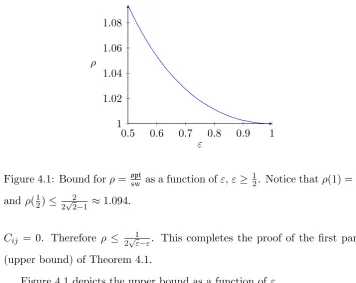
4.1 Additive ε-Nash equilibria with near optimal social welfare . 73
4.2 New contributions . . . 74
4.3 Preliminaries . . . 76
4.4 Approximation withε≥ 1
2 . . . 77 4.5 Upper bound in Theorem 4.1 . . . 80
4.6 Lower bound in Theorem 4.1 . . . 82
4.7 Win-lose games withε≥ 1
2 . . . 83 4.8 Approximation withε < 12 . . . 84
4.9 Reducing social welfare . . . 85
4.10 Analysis of the case opt≥ 2−3ε
1−ε . . . 86
5 Plutocratic and egalitarian ε-NE 91
5.1 Preliminaries . . . 96
5.2 Approximate Plutocratic NE . . . 97
5.2.1 The First Case: ε≥ 12 . . . 98
5.2.2 The Second Case: 3−
√
5 2 ≤ε <
1
2 . . . 102
5.3 Approximate Egalitarian NE . . . 107
5.3.1 The First Case: ε≥1/2 . . . 107
5.3.2 The Second Case: 3−
√
5 2 ≤ε <
1
2 . . . 110
III Communication complexity of approximate Nash
equi-libria 115
6 Communication complexity 117
6.1 How to communicate mixed strategies . . . 119
6.2 Communication-efficient additive 0.382-Nash
6.3 Communication-efficient additive 23
-well-supported Nash equilibria . . . 123
Introduction
John Nash proved that everyfinite game (finite number of players and finite
number of strategies) has at least one Nash equilibrium [45]. This is a
guarantee that every finite game has at least one strategy profile that no
player has any incentive to deviate from. But, can we compute a Nash
equilibrium efficiently?
The problem of computing Nash equilibria is one of the most
fundamen-tal problems in algorithmic game theory. There were a lot of attempts to
find a polynomial-time algorithm for computing Nash equilibria, with the
most notable one the Lemke-Howson algorithm [41], a method to find a
Nash equilibrium for two-player games. Unfortunately, it was proved that
this algorithm has exponential worst-case performance [50]. Furthermore, it
is now known that the problem of computing a Nash equilibrium isPPAD -complete [21], even for two-player games [10]. Given this evidence of
in-tractability of the problem, further research has focused on the
computa-tion ofapproximate Nash equilibria. In this context—and assuming that all
payoffs are normalized to be in the [0,1] interval1—the standard notions of
1
It is easy to see that the set of the Nash equilibria of normal-form games is invariant under additive and positive multiplicative transformations of the payoff matrices.
approximation are the additive or relative approximation with a parameter
ε∈ [0,1]. There are two different variants of additive/relative
approxima-tion of Nash equilibria: the ε-Nash equilibrium and the ε-well-supported
Nash equilibrium.
An additive ε-Nash equilibrium is a strategy profile—one strategy for
each player—in which no player can improve her payoff by more than ε
through unilateral deviation from her strategy in the strategy profile.
Sev-eral polynomial-time algorithms have been proposed to find additiveε-Nash
equilibria in bimatrix games for ε = 3/4 by Kontogiannis et al. [37], for
ε= 1/2 and for ε = (3−√5)/2 ≈ 0.382 by Daskalakis et al. [23, 22], for
ε= 1/2−1/(3√6)≈0.364 by Bosse et al. [7], and finally forε≈0.3393 by
Tsaknakis and Spirakis [51]. Also, a polynomial-time algorithm for additive
(1/3 +δ)-Nash equilibria, for any δ > 0, was given for symmetric
bima-trix games by Kontogiannis and Spirakis [39]. For more than two players,
there is a polynomial-time algorithm to give additive mm−1-Nash
equilib-ria, where m is the number of players, and a recursive method to give an
additive
1 2−α
-Nash equilibrium formplayers if we can find an additiveα
-Nash equilibrium form−1 players (see [7, 9, 35]). Furthermore, Deligkas et
al. gave a polynomial-time algorithm for computing additive (1/2 +δ)-Nash
equilibria for polymatrix games [25], for anyδ >0. It is also known the
exis-tence of additiveε-Nash equilibria in normal-form games with support of size
O((logm+ logn−logε)/ε2) for arbitrarily small ε > 0 [42, 35, 5], where
n is the number of pure strategies. This implies a quasi-polynomial-time
algorithm for games with constant number of players. For lower bounds, by
Feder et al. [28] it is known that, for anyε <1/2, poly-logarithmic supports
of strategies are needed in order to find an additive ε-Nash equilibrium in
ε-Nash equilibrium for some constantε >0 isPPAD-complete for the classes of polymatrix and degree 3 graphical games, in which each player has only
two strategies. Recently, Rubinstein [49] has provided evidence that there is
a constant ε >0, such that computing ε-Nash equilibria in bimatrix games
in time significantly better than the algorithm of [42] may not be possible.
An additive ε-well-supported Nash equilibrium is a strategy profile in
which the expected payoff of any pure strategy that is used in a mixed
strategy of a player is at most ε less than the expected payoff of the
best-response strategy (strategy that maximizes the expected payoff). It is a
notion stronger than that of an additiveε-Nash equilibrium: every additive
ε-well-supported Nash equilibrium is also an additive ε-Nash equilibrium,
but not necessarily vice-versa. The smallestε for which a polynomial-time
algorithm is currently known that computes an additive ε-well-supported
Nash equilibrium in an arbitrary bimatrix game is 0.6528 [38, 26, 27, 13]. By
Kontogiannis and Spirakis [38] we know that one can find additive 1/
2-well-supported Nash equilibria for the special class of win-lose bimatrix games in
polynomial-time. Also, by Czumaj et al. [16] we know how to find an
addi-tive (1/2+δ)-well-supported Nash equilibrium in symmetric bimatrix games,
for anyδ >0, in polynomial-time. Furthermore, the quasi-polynomial-time
algorithm for additive ε-Nash equilibria is also applied to additive ε
-well-supported Nash equilibria in bimatrix games, so it is known how to find
ad-ditiveε-well-supported Nash equilibria in quasi-polynomial timenO(logn/ε2)
for arbitrarily small ε >0 [38]. On the negative side, poly-logarithmic
sup-ports of strategies are required for additiveε-well-supported Nash equilibria
[3, 2], for anyε <1.
Our knowledge for relative approximations is limited. While the notion
in the past, significantly less attention has been paid to the notion of the
relative approximate Nash equilibria: relativeε-Nash equilibria and relative
ε-well-supported Nash equilibria. Any relative approximate Nash equilibrium
is also an additive approximate Nash equilibrium, but not vice-versa. A
relativeε-Nash equilibrium is a strategy profile in which the payoff of each
player is at least (1−ε) times the payoff of the best-response strategy. Most
of the relevant results we are aware of appeared in the paper of Feder et al.
[28] for bimatrix games. On the positive side, Feder et al. [28, Theorem 3]
give a polynomial-time algorithm that finds a relative ε-Nash equilibrium
for ε slightly smaller than 12. (There exists a function f(n) = (2 +o(1))n
such that for any α, 0 < α < 8nf1(n), one can find in polynomial-time a
relative (12 −α)-Nash equilibrium; the relative (12 −α)-Nash equilibrium
found is a pure row strategy and a mixed column strategy.) On the negative
side, Feder et al. [28, Theorem 1] show that for any α, 0 < α ≤ 1 2, if one limits the column player to strategies with support of size less than
log2n
log2(1/α), then it is not possible to find a relative ( 1
2 −α)-Nash equilibrium, even for constant-sum 0/1 games. Furthermore, Feder et al. [28, Theorem
2] show bimatrix constant-sum 0/1 games for which for any ε, 0 < ε < 12,
no pair of mixed strategies with supports of size smaller thanO(ε−2logn)
has a relative ε-Nash equilibrium. Further, in a related work, Daskalakis
[20] considers the notion of a relative ε-well-supported Nash equilibrium,
a strategy profile in which any pure strategy that is played by the players
has payoff at least (1−ε) times the best-response payoff. He shows that the
problem of finding a relativeε-well-supported Nash equilibrium in two-player
games, with payoff values in [−1,1], is PPAD-complete, even for constant values of approximation in some bimatrix games. Finally, in [48] Aviad
-well-supported Nash equilibrium in a bimatrix game with positive payoffs is
PPAD-complete for constant values of approximation.
1.1
New contributions
In this thesis our main goal is a new study of the complexity of various
variants of the approximate Nash equilibrium. In Chapter 2, we study
polynomial-time algorithms for additive approximate Nash equilibria in
bi-matrix and multi-player games. Specifically, we present new techniques
based on zero-sum games and their applications to additive approximate
Nash equilibria in bimatrix games. Then, we present a polynomitime
al-gorithm to compute additive 23-well-supported Nash equilibria in bimatrix
games and a polynomial-time algorithm to compute additive (12 +δ
)-well-supported Nash equilibria in symmetric bimatrix games, for anyδ >0. At
the end of this chapter, we study polynomial-time algorithms of additive
approximate Nash equilibria in multi-player games. Results presented in
this chapter are also presented in [13, 16, 14, 15].
In Chapter 3, we investigate algorithms for relative approximate Nash
equilibria. We first present a polynomial-time algorithm for computing
rela-tive 1/2-Nash equilibria in bimatrix games and then we generalize this result
to multi-player games. Results of Chapter 3 are also presented in [14].
In Chapter 4, we study polynomial-time algorithms for computing
ad-ditive ε-Nash equilibria in bimatrix games that are also close to the social
welfare of the game. Results of Chapter 4 are also presented in [17].
In Chapter 5, we study polynomial-time algorithms for computing
ad-ditiveε-Nash equilibria in bimatrix games that are also close to variants of
the social welfare of any Nash equilibrium of the game. Results of Chapter
Finally, in Chapter 6 we study the communication complexity of
addi-tive approximate Nash equilibria in bimatrix games. We give an algorithm
to compute an additive (0.382 +δ)-Nash equilibrium and an algorithm to
compute an additive (2/3 +δ)-well-supported Nash equilibrium in bimatrix
games under the communication complexity constraint for anyδ >0. Some
parts of this chapter are also presented in [13].
1.2
Definitions — bimatrix games
We consider bimatrix games (R, C), whereR, C∈[0,1]n×nare the matrices
of payoffs for the two players: the row player and the column player,
respec-tively. If the row player uses a strategyi, 1≤i≤n, and if the column one
uses a strategyj, 1≤j≤n, then the row player receives payoffRij and the
column player receives payoffCij.
Let ∆ = {x ∈ [0,1]n : Pn
i=1x(i) = 1} be the set of mixed strategies: amixed strategy xis a probability distribution on the set of pure strategies
{1,2, . . . , n}. If the row player uses a mixed strategy x and the column
player uses a mixed strategy y, then the row player receives payoff xTRy
and the column player receives payoff xTCy. A pair of strategies (x, y),
the former for the row player and the latter for the column player, is often
referred to as a strategy profile. We define the support supp(x) of a mixed
strategyxto be the set of pure strategies that have positive probability inx,
i.e., supp(x) ={i : 1≤i≤nand x(i) >0}. Letei be the mixed strategy
such that a player plays the pure strategyi, in other wordsei is the column
vector that has 1 in the coordinate i and 0 elsewhere. We define M(Ry)
the set of the pure best-response strategies (pure strategies that maximize
the expected payoff) of the row player against the strategyy of the column
column player against the strategy x of the row player.
For every i, 1 ≤ i ≤n, let Ri• be the row vector of the payoffs of the
payoff matrix R when the row player uses the strategyi, or in other words
eT
i R. Note that if the row player uses a pure strategy i, 1 ≤ i ≤ n, and if the column player uses a mixed strategy y, then the row player receives
payoff Ri•y, or equivalently eTiRy. Similarly, for every j, 1 ≤ j ≤ n, let
C•j be the column vector of the payoffs of the matrix C when the column
player uses the strategy j, or in other words Cej. Note that if the column
player uses a pure strategyj, 1≤j≤n, and if the row player uses a mixed
strategy x, then the column player receives payoff xTC•j, or equivalently
xTCej.
We define fR(x, y)—the row regret of (x, y)—byfR(x, y) = max(Ry)−
xTRy, where max(Ry) = maxi(eTi Ry) and fC(x, y) —the column regret
of (x, y)—byfC(x, y) = max(xTC)−xTCy, where max(xTC) = maxj(xTCej).
We define the maximumregret f(x, y) of a strategy profile (x, y) byf(x, y) =
max{fR(x, y), fC(x, y)}. We have the following definitions.
Definition 1.1 (Nash equilibrium (NE)) ANash equilibriumis a
strat-egy profile(x∗, y∗) such that
• for everyi, 1≤i≤n, we have Ri•y∗ ≤(x∗)TRy∗, and
• for everyj, 1≤j≤n, we have (x∗)TC•j ≤(x∗)TCy∗,
or, in other words, if x∗ is a best-response strategy to y∗ and y∗ is a
best-response strategy to x∗.
Proposition 1.2 (Nash equilibrium) A strategy profile(x∗, y∗)is a Nash
equilibrium if and only if f(x∗, y∗) = 0, or, in other words, the maximum
Definition 1.3 (Additive ε-Nash equilibrium) For everyε >0, an
ad-ditiveε-Nash equilibrium is a strategy profile (x∗, y∗) such that
• for everyi,1≤i≤n, we haveRi•y∗−(x∗)TRy∗ ≤ε, and
• for everyj,1≤j ≤n, we have (x∗)TC
•j−(x∗)TCy∗≤ε,
or, in other words, if x∗ is an ε-best-response strategy to y∗ and y∗ is an
ε-best-response strategy to x∗.
Proposition 1.4 (Additive ε-Nash equilibrium) A strategy profile(x∗,
y∗)is anadditiveε-Nash equilibriumif and only iff(x∗, y∗)≤ε,or, in other
words, the maximum regret of the players is at mostε.
Note that an additive 0-Nash equilibrium is an exact Nash equilibrium.
Definition 1.5 (Additive ε-well-supported Nash equilibrium) For
e-very ε > 0, an additive ε-well-supported Nash equilibrium is a strategy
profile(x∗, y∗) such that
• for every i, 1≤i≤n, and i0 ∈supp(x∗), we have Ri•y∗−Ri0•y∗ ≤ε,
and
• for every j, 1 ≤ j ≤ n, and j0 ∈ supp(y∗), we have (x∗)TC•j −
(x∗)TC
•j0 ≤ε,
or, in other words, if everyi0 ∈supp(x∗)is anε-best-response strategy toy∗
and every j0 ∈supp(y∗) is an ε-best response strategy to x∗.
Note that any additive ε-well-supported Nash equilibrium is an additive ε
-Nash equilibrium and that an additive 0-well-supported Nash equilibrium is
Definition 1.6 (Relative ε-Nash equilibrium) For every ε > 0, a
rel-ativeε-Nash equilibrium2 is a strategy profile (x∗, y∗) such that
• for everyi, 1≤i≤n, we have (x∗)TRy∗ ≥(1−ε)·Ri•y∗, and
• for everyj, 1≤j≤n, we have (x∗)TCy∗ ≥(1−ε)·(x∗)TC•j.
Note that a relative 0-Nash equilibrium is an exact Nash equilibrium.
Definition 1.7 (Relative ε-well-supported Nash equilibrium) For
e-veryε >0, a relativeε-well-supported Nash equilibriumis a strategy profile
(x∗, y∗) such that
• for every i, 1 ≤ i ≤n, and i0 ∈ supp(x∗), we have (1−ε)·Ri•y∗ ≤
Ri0•y∗, and
• for everyj,1≤j≤n, and j0 ∈supp(y∗), we have(1−ε)·(x∗)TC•j ≤
(x∗)TC•j0.
Note that anyrelativeε-well-supported Nash equilibrium is arelativeε-Nash
equilibriumand that a relative 0-well-supported Nash equilibrium is an exact
Nash equilibrium.
Definition 1.8 (Win-lose game) A game is win-lose if any payoff entry
belongs in {0,1}.
Definition 1.9 (Symmetric game, symmetric Nash equilibrium) A
bimatrix game (R, C) is symmetric if C=RT.
2
Let us note that we use the definition from Daskalakis in [20] that is consistent with the notion of the additiveε-Nash equilibria, but it differs from the definition from Feder et al. [28], where one replaced the (1−ε) factor byε. That is, the definition in Feder et al. [28] for two players was that a strategy profile (x, y) is a“Feder-et-al.”-relativeα-Nash equilibrium ifxTRy≥α·(x0)TRyandxTCy≥α·xTCy0for all mixed strategiesx0 and
A symmetric Nash equilibrium in a symmetric bimatrix game (R, RT)
is a strategy profile (x∗, x∗) such that for every i, 1 ≤ i ≤ n, we have
Ri•x∗≤(x∗)TRx∗. Note that then it also follows that for everyj,1≤j≤n,
we have:
(x∗)TRT•j =Rj•x∗ ≤(x∗)TRx∗ = (Rx∗)Tx∗ = (x∗)TRTx∗.
Let us recall a fundamental theorem of John Nash [45] about existence
of symmetric Nash equilibria in symmetric games.
Theorem 1.10 (John Nash [45]) Every finite symmetric game has a
sym-metric Nash equilibrium.
Now we will describe a general lemma for the additiveε-Nash equilibria
which has been used in all the previous algorithms that guarantee additive
ε-Nash equilibria (see [37, 7, 22, 23, 51]).
Lemma 1.11 Let (x1, y) and (x2, y) be two strategy profiles, with row
re-grets fR(x1, y), fR(x2, y) and column regrets fC(x1, y), fC(x2, y). Any
con-vex combination between these two strategy profiles has regrets no larger than
the convex combination of the regrets.
Proof. Consider a convex combination (px1+ (1−p)x2, y), for some p ∈
[0,1]. Then, the regret of the row player is:
fR(px1+ (1−p)x2, y) = max(Ry)−(px1+ (1−p)x2)TRy
= max(Ry)−p(x1)TRy−(1−p)(x2)TRy
=pmax(Ry) + (1−p) max(Ry)−p(x1)TRy−(1−p)(x2)TRy
=pfR(x1, y) + (1−p)fR(x2, y),
The regret of the column player is:
fC(px1+ (1−p)x2, y) = max((px1+ (1−p)x2)TC)−(px1+ (1−p)x2)TCy
≤pmax((x1)TC) + (1−p) max((x2)TC)−p(x1)TCy−(1−p)(x2)TCy
=pfC(x1, y) + (1−p)fC(x2, y),
sincefC(x1, y) = max((x1)TC)−(x1)TCy, andfC(x2, y) = max((x2)TC)−
(x2)TCy. ut
We now give a definition that we use it to prove additive ε-well-supported
Nash equilibria.
Definition 1.12 (Preventing exceeding payoffs) We say that a
strat-egy x ∈[0,1]n for the row player prevents exceeding u ∈ [0,1] if for every
j= 1,2, . . . , n, we have xTC•j ≤u or, in other words, if the column player
payoff of the best-response strategy tox does not exceedu. Similarly, we say
that a strategy y∈[0,1]nfor the column player prevents exceeding v∈[0,1]
if for every i= 1,2, . . . , n, we have Ri•y≤v or, in other words, if the row
player payoff of the best-response strategy to y does not exceed v.
For brevity, we say that a strategy profile (x, y) prevents exceeding (v, u)
if x prevents exceeding u andy prevents exceeding v.
Observe that the following system of linear constraints PE(v, u)
charac-terizes strategy profiles (x, y) that prevent exceeding (v, u)∈[0,1]2:
n
X
i=1
x(i) = 1; x(i)≥0 for alli= 1,2, . . . , n;
n
X
j=1
y(j) = 1; y(j)≥0 for all j= 1,2, . . . , n;
Ri•y≤v for all i= 1,2, . . . , n;
Note that if (x, y) is a Nash equilibrium then, by definition, it prevents
exceeding (xTRy, xTCy), which implies the following Proposition.
Proposition 1.13 If (x, y) is a Nash equilibrium, v ≥ xTRy, and u ≥
xTCy, then PE(v, u) has a solution and it prevents exceeding(v, u).
By the following proposition, in order to find an additiveε-well-supported
Nash equilibrium it suffices to find a strategy profile that prevents exceeding
(ε, ε).
Proposition 1.14 If a strategy profile (x, y) prevents exceeding(v, u) then
it is an additivemax(v, u)-well-supported Nash equilibrium.
Proof. Let i0∈supp(x) and leti∈ {1,2, . . . , n}. Then we have:
Ri•y−Ri0•y≤Ri•y≤v,
where the first inequality follows from Ri0•y ≥ 0, and the other one holds
because y prevents exceeding v. Similarly, and using the assumption that
x prevents exceeding u, we can argue that for all j0 ∈ supp(y) and j ∈
{1,2, . . . , n}, we have xTC•j − xTC•j0 ≤ u. It follows that (x, y) is a
max(v, u)-well-supported Nash equilibrium. ut
We now introduce another definition which we also use to prove additive
ε-well-supported Nash equilibria.
Definition 1.15 (Well supporting payoffs) We say that a strategy x ∈
[0,1]n for the row player well supportsv∈[0,1]against a strategyy∈[0,1]n
for the column player if for everyi∈supp(x), we haveRi•y≥v. Similarly,
we say that a strategy y ∈ [0,1]n for the column player well supports u ∈
[0,1]against a strategyx∈[0,1]nfor the row player if for everyj∈supp(y),
For brevity, we say that a strategy profile (x, y) well supports (v, u) if x
well supports v against y and y well supports u againstx.
By the following proposition, in order to find an additiveε-well-supported
Nash equilibrium it suffices to find a strategy profile that well supports
(1−ε,1−ε).
Proposition 1.16 If a strategy profile (x, y) well supports (v, u) then it is
an additive max(1−v,1−u)-well-supported Nash equilibrium.
Proof. Leti0 ∈supp(x) and let i∈ {1,2, . . . , n}. Then we have:
Ri•y−Ri0•y≤Ri•y−v≤1−v,
where the first inequality follows from Ri0•y ≥v, and the other one holds
because Ri•y ≤1. Similarly, for the column player. It follows that (x, y) is
a max(1−v,1−u)-well-supported Nash equilibrium. ut
We now define zero-sum bimatrix games and we present some properties
of them that we use to find additive approximate Nash equilibria.
Definition 1.17 (Zero-sum game) A bimatrix game (R, C) ∈ Rn×n is
zero-sum if and only if C=−R.
Note that we can compute exact Nash equilibria in polynomial-time in
zero-sum games using linear programming.
Let (A,−A) be a zero-sum game with Nash equilibrium (x, y) and value
v=xTAy. Then, by the definition of the Nash equilibrium we know that
• for everyi, 1≤i≤n, we have Ai•y ≤v, and
we can see that y prevents exceeding v. Let (−A, A) be a zero-sum game
with Nash equilibrium (x, y) and value u =xTAy. Then, by the definition
of the Nash equilibrium we know that
• for everyi, 1≤i≤n, we have Ai•y≥u, and
• for everyj, 1≤j ≤n, we have (x)TA
•j ≤u,
we can see thatxprevents exceeding u.
1.3
Definitions — multiplayer games
Consider a normal-form game withm players. Each player has nstrategies
at the disposal and the entries of the payoff matrices are in [0,1]. A mixed
strategy x∈[0,1]n is a column vector that describes a probability
distribu-tion on thenpure strategies of a player; a support of a mixed strategyx is
the set of the pure strategies k such that x(k) > 0. We write x−i for the
strategy profile of all players except for the playeri. If the player iplays a
mixed strategy xi, then the expected payoff of the playeriis ui(xi, x−i).
A Nash equilibrium is any strategy profile x = (xi, x−i) such that if
every player randomizes according tox, then no player has an incentive to
change her mixed strategy. More formally, a strategy profile x = (xi, x−i)
is a Nash equilibrium if and only if for everyi ui(xi, x−i) ≥ui(x0i, x−i), for
every mixed strategy x0i. Equivalently, a strategy profile x = (xi, x−i) is a
Nash equilibrium if and only if for all players i
ui(xi, x−i)≥ui(ek, x−i) for everyk= 1, . . . , n,
where ek represents the unit vector along dimension k of Rn, that is, ek ∈
As in bimatrix games, there are two main models of approximate Nash
equilibria studied in the literature, one focusing on the additive quality
in-centive and another concerned with the relative quality incentive. We will
describe the additive/relativeε-Nash equilibrium, assuming that the payoff
matrices of the players have all entries in [0,1].
For any ε ≥ 0, an additive ε-Nash equilibrium is any strategy profile
x = (xi, x−i) such that for every player i ui(xi, x−i) ≥ ui(x0i, x−i)−ε, for
every strategyx0i. Equivalently, a strategy profilex= (xi, x−i) is an additive
ε-Nash equilibrium if for every playeri
ui(xi, x−i)≥ui(ek, x−i)−ε for everyk= 1, . . . , n.
Note that an additive 0-Nash equilibrium is a Nash equilibrium.
For any ε ≥ 0, a relative ε-Nash equilibrium is any strategy profile x =
(xi, x−i) such that for every playeri ui(xi, x−i)≥ui(x0i, x−i)−ε·ui(x0i, x−i) =
(1−ε)·ui(x0i, x−i), for every mixed strategyx0i. Equivalently, for anyε≥0,
a strategy profile x = (xi, x−i) is a relative ε-Nash equilibrium if and only
if for every player i
ui(xi, x−i)≥(1−ε)·ui(ek, x−i) for every k= 1, . . . , n.
Part I
Algorithms for approximate
Nash equilibria
Chapter 2
Additive approximate Nash
equilibria
In this chapter, we study algorithms for additive approximate Nash
equi-libria. We first describe the state-of-art for additive ε-Nash equilibria in
bimatrix games, the Tsaknakis-Spirakis algorithm [51]. Then, we present
new techniques that are based on zero-sum games and their applications
to additive approximate Nash equilibria in bimatrix games. After this we
present methods to compute additive 23-well-supported Nash equilibria in
arbitrary bimatrix games and additive (12+δ)-well-supported Nash
equilib-ria in symmetric bimatrix games, for anyδ >0. Finally, we study issues of
additive approximate Nash equilibria in multi-player games.
2.1
Tsaknakis-Spirakis algorithm
In this section we will describe the Tsaknakis-Spirakis algorithm [51] for
computing additive 0.3393-Nash equilibria, the state-of-art for computing
additive ε-Nash equilibria in bimatrix games.
2.1.1 Directional Derivative of Regret
Our main interest in this section is to identify and study the properties
of stationary points of the regret function on the set of strategy profiles,
because—as observed by Tsaknakis and Spirakis [51], and as we elaborate
later—they are crucial to obtain additiveε-Nash equilibria with low regret.
Let (x, y),(x0, y0)∈∆2 be strategy profiles, and letf be the regret
func-tion as it was defined in the Chapter 1. We define thedirectional derivative
of f at (x, y) towards (x0, y0) by:
∇(x0,y0)f(x, y) = lim
ε&0 f
(1−ε)(x, y) +ε(x0, y0)
−f(x, y)
ε ,
if the limit exists.
Lemma 2.1 [51] For all strategy profiles (x, y) and (x0, y0), the directional
derivative ∇(x0,y0)f(x, y) is well defined. More specifically, we have: If
fR(x, y)> fC(x, y) then
∇(x0,y0)f(x, y) =∇(x0,y0)fR(x, y) =
max
M(Ry)(Ry
0)−xTRy0−(x0)TRy+xTRy−f
R(x, y),
and if fR(x, y)< fC(x, y) then
∇(x0,y0)f(x, y) =∇(x0,y0)fC(x, y) =
max
M(xTC) (x
0)TC
If fR(x, y) =fC(x, y) then
∇(x0,y0)f(x, y) = max n
∇(x0,y0)fR(x, y),∇(x0,y0)fC(x, y) o
.
Proof. Recall that M(Ry) (as defined in Chapter 1) is the set of the pure
best-response strategies of the row player to the mixed strategy y of the
column player, and the complement of M(Ry) is M(Ry) = {1, . . . , n} \
M(Ry). Also,M(xTC) is the set of the pure best-response strategies of the
column player to strategyxof the row player. The complement ofM(xTC)
is M(xTC) ={1, . . . , n} \ M(xTC). The difference of the regrets between
the points (1−ε)(x, y) +ε(x0, y0) and (x, y) is equal to
f
(1−ε)(x, y) +ε(x0, y0)
−f(x, y) =
= maxnfR
(1−ε)(x, y) +ε(x0, y0), fC
(1−ε)(x, y) +ε(x0, y0)o
−f(x, y) = maxnfR
(1−ε)(x, y) +ε(x0, y0)−f(x, y),
fC
(1−ε)(x, y) +ε(x0, y0)
−f(x, y)
o
.
With this at hand and by the definition of the directional derivative of the
regret function we have that the directional derivative of the regret function
is equal to
∇(x0,y0)f(x, y) = max n
lim ε&0
fR
(1−ε)(x, y) +ε(x0, y0)
−f(x, y)
ε ,
lim ε&0
fC
(1−ε)(x, y) +ε(x0, y0)
−f(x, y)
ε
o
We analyse the part
lim ε&0
fR
(1−ε)(x, y) +ε(x0, y0)−f(x, y)
ε ,
since the other part is analogous. First we will analyse the part fR
ε)(x, y) +ε(x0, y0)
, so this part is equal to
fR
(1−ε)(x, y) +ε(x0, y0)=
= max
R
(1−ε)y+εy0
−(1−ε)x+εx0
T
R
(1−ε)y+εy0
= maxR(1−ε)y+εy0−(1−ε)2xTRy−ε(1−ε)xTRy0
−ε(1−ε)(x0)TRy−ε2(x0)TRy0 = max
R
(1−ε)y+εy0
−xTRy−ε2xTRy+ 2εxTRy−εxTRy0+ε2xTRy0
−ε(x0)TRy+ε2(x0)TRy−ε2(x0)TRy0.
However, we can write up the maxR(1−ε)y+εy0as
maxR(1−ε)y+εy0=
= max
M(Ry)
R(1−ε)y+εy0+ maxn0, max
M(Ry)
R(1−ε)y+εy0
− max
M(Ry)
R(1−ε)y+εy0o.
So, we have that
fR
(1−ε)(x, y) +ε(x0, y0)
=
= max
M(Ry)
R(1−ε)y+εy0+ maxn0, max
M(Ry)
R(1−ε)y+εy0
− max
M(Ry)
R
(1−ε)y+εy0
o
−xTRy−ε2xTRy+ 2εxTRy
−εxTRy0+ε2xTRy0−ε(x0)TRy+ε2(x0)TRy−ε2(x0)TRy0. (2.1)
We can see that lim ε&0max
n
0,maxM(Ry)R(1−ε)y+εy0−maxM(Ry)
R
(1−ε)y+εy0o= 0,since lim
ε&0maxM(Ry)
R(1−ε)y+εy0−maxM(Ry)
R
(1−ε)y+εy0
that they are not best-responses toy. Thus, we summarize that
lim ε&0
fR
(1−ε)(x, y) +ε(x0, y0)−f(x, y)
ε =
= lim ε&0
maxM(Ry)
R
(1−ε)y+εy0
−xTRy−ε2xTRy+ 2εxTRy
ε
−εxTRy0+ε2xTRy0−ε(x0)TRy+ε2(x0)TRy−ε2(x0)TRy0−f(x, y)
ε
= lim ε&0
maxM(Ry)
R(1−ε)y+εy0−xTRy+ 2εxTRy−εxTRy0
ε
−ε(x0)TRy−f(x, y)
ε = limε&0
(1−ε) maxM(Ry)(Ry) +εmaxM(Ry)(Ry0) ε
−xTRy+ 2εxTRy−εxTRy0−ε(x0)TRy−f(x, y)
ε ,
the second equality holds since lim ε&0
−ε2xTRy+ε2xTRy0+ε2(x0)TRy−ε2(x0)TRy0
ε = 0.
The third equality holds by the property of maxM(Ry)
R(1−ε)y+εy0=
(1−ε) maxM(Ry)(Ry) +εmaxM(Ry)(Ry0),in which the equality holds since
every strategy in M(Ry) is a pure best-response strategy to y, so has the
same expected payoff against y. We have three cases: fR(x, y) > fC(x, y),
fR(x, y) =fC(x, y), andfR(x, y)< fC(x, y).
• IffR(x, y)> fC(x, y),
lim ε&0
fC
(1−ε)(x, y) +ε(x0, y0)
−f(x, y)
ε =
= lim ε&0
fC
(1−ε)(x, y) +ε(x0, y0)
−fR(x, y)
ε =−∞,
sincef(x, y) =fR(x, y)> fC(x, y), and
lim ε&0
fR
(1−ε)(x, y) +ε(x0, y0)
−f(x, y)
ε =
= max
M(Ry)(Ry
0
)−(x0)TRy−xTRy0+xTRy−fR(x, y)
= max
M(Ry)(Ry
0
The first equality holds since maxM(Ry)(Ry) = max(Ry) and the
sec-ond equality holds sincef(x, y) =fR(x, y).
• IffR(x, y)< fC(x, y),
lim ε&0
fR
(1−ε)(x, y) +ε(x0, y0)
−f(x, y)
ε =
= lim ε&0
fR
(1−ε)(x, y) +ε(x0, y0)
−fC(x, y)
ε =−∞,
sincef(x, y) =fC(x, y)> fR(x, y), and
lim ε&0
fC
(1−ε)(x, y) +ε(x0, y0)−f(x, y)
ε =
= max
M(xTC)((x
0
)TC)−(x0)TCy−xTCy0+xTCy−fC(x, y)
= max
M(xTC)((x
0)TC)−(x0)TCy−xTCy0+xTCy−f(x, y).
The first equality holds since maxM(xTC)(xTC) = max(xTC) and the
second equality holds sincef(x, y) =fC(x, y).
• IffR(x, y) =fC(x, y),
lim ε&0
fR
(1−ε)(x, y) +ε(x0, y0)−f(x, y)
ε =
= max
M(Ry)(Ry
0
)−(x0)TRy−xTRy0+xTRy−fR(x, y)
= max
M(Ry)(Ry
0
)−(x0)TRy−xTRy0+xTRy−f(x, y).
The first equality holds since maxM(Ry)(Ry) = max(Ry) and the
sec-ond equality holds sincef(x, y) =fR(x, y).
lim ε&0
fC
(1−ε)(x, y) +ε(x0, y0)
−f(x, y)
ε =
= max
M(xTC)((x
0
)TC)−(x0)TCy−xTCy0+xTCy−fC(x, y)
= max
M(xTC)((x
The first equality holds since maxM(xTC)(xTC) = max(xTC) and the
second equality holds sincef(x, y) =fC(x, y).
We summarize, so in total we have that
• IffR(x, y)> fC(x, y),
∇(x0,y0)f(x, y) =
= max
n
max
M(Ry)(Ry
0)−(x0)TRy−xTRy0+xTRy−f(x, y),−∞o
= max
M(Ry)(Ry
0)−(x0)TRy−xTRy0+xTRy−f(x, y).
• IffR(x, y)< fC(x, y),
∇(x0,y0)f(x, y) =
= max
n
− ∞, max
M(xTC)
(x0)TC
−(x0)TCy−xTCy0+xTCy−f(x, y)
o
= max
M(xTC)
(x0)TC−(x0)TCy−xTCy0+xTCy−f(x, y).
• IffR(x, y) =fC(x, y),
∇(x0,y0)f(x, y) =
= maxn max
M(Ry)(Ry
0)−(x0)TRy−xTRy0+xTRy−f(x, y),
max
M(xTC)
(x0)TC−(x0)TCy−xTCy0+xTCy−f(x, y)o
= max
n
max
M(Ry)(Ry
0
)−(x0)TRy−xTRy0+xTRy,
max
M(xTC)
(x0)TC
−(x0)TCy−xTCy0+xTCy
o
−f(x, y).
u t
We now give a definition of the stationary andδ-stationary points of the
Definition 2.2 A strategy profile (x, y) is a stationary point of the
re-gret function f if and only if for every strategy profile (x0, y0) we have
∇(x0,y0)f(x, y)≥0.
Definition 2.3 A strategy profile(x, y) is aδ-stationary point of the regret
function f if and only if for any δ ∈ [0,1] and for every strategy profile
(x0, y0) we have ∇(x0,y0)f(x, y)≥ −δ.
Note that any 0-stationary point is a stationary point of the function.
Lemma 2.4 If(x, y) is a stationary point of the regret functionf, then the
regrets of the players at the point (x, y) are equal.
Proof. Let (x, y) be a stationary point with not equal regrets, we assume
without loss of generality thatfR(x, y)> fC(x, y). We consider a direction
of (x0, y), where x0 is a best-response strategy to y. Since, we are in a
stationary point the directional derivative in this point for this direction is
non-negative, ∇(x0,y)f(x, y)≥0, so we have that
max
M(Ry)(Ry)
−(x0)TRy−xTRy+xTRy−fR(x, y)≥0,
this implies thatfR(x, y)≤maxM(Ry)(Ry)−(x0)TRy= 0,since (x0)TRy=
max(Ry) = maxM(Ry)(Ry), since x0 is a best-response toy. But, by
defini-tion fC(x, y)≥0, so we have that 0> fC(x, y)≥0, this is a contradiction.
u t
2.1.2 An LP for Minimizing Directional Derivative
We present a linear program that—for a given strategy profile (x, y)—yields
regret function∇(x0,y0)f(x, y) is minimized.
minimizeγ (2.2)
s.t. x0(i)≥0, y0(j)≥0 1≤i, j≤n (2.3) n
X
i=1
x0(i) = 1,
n
X
j=1
y0(j) = 1 (2.4)
γ≥Ri•y0−(xTR)y0−(Ry)Tx0+xTRy i∈ M(Ry) (2.5)
γ≥C•Tjx0−(xTC)y0−(Cy)Tx0+xTCy j∈ M(xTC) (2.6)
Henceforth we refer to this linear program asthe primal.
Consider the dual linear program, with dual variables a and b,
respec-tively, corresponding to primal constraints (2.4); dual variables pi, for all
i ∈ M(Ry), corresponding to primal constraints (2.5); and dual variables
qj, for all j∈ M(xTC), corresponding to primal constraints (2.6).
maximizeP·xTRy+Q·xTCy+a+b (2.7)
s.t. pi ≥0 i∈ M(Ry)
(2.8)
qj ≥0 j ∈ M(xTC)
(2.9)
P = X
i∈M(Ry)
pi, Q=
X
j∈M(xTC)
qj (2.10)
P+Q= 1 (2.11)
a≤ X
i∈M(Ry)
−(Ry)kpi+
X
j∈M(xTC)
[−(Cy)k+Ckj]qj 1≤k≤n
(2.12)
b≤ X
j∈M(xTC)
−(xTC)lqj+
X
i∈M(Ry)
[−(xTR)l+Ril]pi 1≤l≤n
Henceforth, we refer to this linear program as the dual. Note that
pri-mal variables x0(k), for all k rows, 1 ≤ k ≤ n, correspond to dual
con-straints (2.12); primal variables y0(l), for all l columns, 1 ≤ l ≤ n,
corre-spond to dual constraints (2.13); and the primal variable γ corresponds to
the dual constraint (2.11). Note that the dual variablesP andQare merely
auxiliary variables (defined by the auxiliary dual constraints (2.10)) that
help unclutter the description of the objective function of the dual linear
program, and its analysis that is to follow.
2.1.3 Intuition behind the dual
We can see that for everyk the constraint
a≤ X
i∈M(Ry)
−(Ry)kpi+
X
j∈M(xTC)
[−(Cy)k+Ckj]qj,
can be written as
a≤ −P·(Ry)k−Q·(Cy)k+Ck•q,
if we divide and multiply withP
j∈M(xTC)qj then we get:
a≤ −P ·(Ry)k−Q·(Cy)k+Q·Ck•z,
where z = q/P
j∈M(xTC)qj is a best-response strategy to x, since j ∈
M(xTC) andqj = 0 forj /∈ M(xTC). It is easy to see that ifPj∈M(xTC)qj = 0, we just omit the last two terms of the inequality.
Similarly, for the other constraints for every l
b≤ X
j∈M(xTC)
−(xTC)lqj +
X
i∈M(Ry)
[−(xTR)l+Ril]pi,
this implies that
we divide and multiply withP
i∈M(Ry)pi then we get
b≤ −Q·(xTC)l−P ·(xTR)l+P ·wTR•l,
wherew=p/P
i∈M(Ry)pi is a best-response strategy toy, sincei∈ M(Ry) andpi = 0 fori /∈ M(Ry). It is easy to see that ifPi∈M(Ry)pi = 0, we just
omit the last two terms of the inequality.
So,the dual maximizes the minimum over all rowsk and all columns l.
For anyk, l we have
P·wTR•l−P·(Ry)k−P·(xTR)l+P·xTRy
+Q·Ck•z−Q·(Cy)k−Q·(xTC)l+Q·xTCy
≥a+b+P ·xTRy+Q·xTCy=γ.
The inequality holds since
−P ·(Ry)k+−Q·(Cy)k+Q·Ck•z≥a,
and
−Q·(xTC)l−P ·(xTR)l+P ·wTR•l≥b.
The equality holds since the value of the primal is equal with the value of
the dual. But we can easily see that for any strategiesx0 andy0 it holds that
P·wTRy0−P·(x0)TRy−P ·xTRy0+P·xTRy
+Q·(x0)TCz−Q·(x0)TCy−Q·xTCy0+Q·xTCy≥γ,
this implies that
P·(wTRy0−(x0)TRy−xTRy0+xTRy)
However, fromthe primal we know that if (x, y) is δ-stationary point then
∇(x0,y0)f(x, y) =γ−f(x, y)≥ −δ,
or, in other words, f(x, y)≤γ+δ.Thus, we conclude that
f(x, y)≤γ+δ≤P ·(wTRy0−(x0)TRy−xTRy0+xTRy)
+Q·((x0)TCz−(x0)TCy−xTCy0+xTCy) +δ, (2.14)
for any direction (x0, y0).
Theorem 2.5 If P or Qis equal to zero, the0-stationary point is an exact
Nash equilibrium.
Proof. We assume without loss of generality thatP = 0. Then, by (2.14)
we have that
f(x, y)≤Q·((x0)TCz−(x0)TCy−xTCy0+xTCy). (2.15)
Then, for the direction (x, y0), where y0 is a best-response strategy to x,
(2.15) becomes
f(x, y)≤Q·(xTCz−xTCy−xTCy0+xTCy) =Q·(xTCz−xTCy0) = 0,
sincez is also a best-response strategy tox. ut
2.1.4 Tsaknakis-Spirakis analysis of stationary points
In this subsection we will describe the analysis of Tsaknakis-Spirakis of
taking approximation bound 0.3393 as it was given in [51]. Let (x, y) be a
0-stationary point. We define
λ= min
y0:supp(y0)⊆M(xTC)(w
and
µ= min
x0:supp(x0)⊆M(Ry)((x 0
)TCz−(x0)TCy). (2.17)
From the support of x0,y0 we can see thaty0 is a best-response strategy to
xand x0 is a best-response strategy toy. For the direction (x, y0) by (2.14)
we get:
f(x, y)≤P ·(wTRy0−xTRy0) =P·λ.
For the direction (x0, y) by (2.14) we get:
f(x, y)≤Q·((x0)TCz−(x0)TCy) =Q·µ.
Sincez is a best-response strategy to x and (2.16) we get:
wTRz−xTRz ≥λ, (2.18)
and since wis a best-response strategy to y and (2.17) we get:
wTCz−wTCy≥µ. (2.19)
Without loss of generality we assume that λ ≥ µ, the analysis in the
caseµ≥λis analogous. Firstly, we analyse the regrets of the two players in
the points (x, z) and (w, z). The regret of the row player in the point (x, z)
isfR(x, z) ≤1,which follows by the fact that max(Rz)≤1. The regret of
the column player isfC(x, z) = 0,since z is a best-response strategy to x.
Now, we analyse the regrets of the players in the point (w, z). The regret of
the row player isfR(w, z) = max(Rz)−wTRz≤1−λ−xTRz≤1−λ,the
first inequality holds since max(Rz)≤1 and (2.18). The second inequality
holds since xTRz ≥ 0. The regret of the column player is fC(w, z) =
max(wTC)−wTCz≤1−µ−wTCy≤1−µ, the first inequality holds since
max(wTC)≤1 and (2.19). The second inequality holds sincewTCy≥0.
Theorem 2.6 The strategy profile 1+λ1−µw+1+λ−λ−µµx, z is an additive
1−µ 1+λ−µ
Proof. The regret of the row player, by Lemma 1.11, is:
fR
1
1 +λ−µw+
λ−µ
1 +λ−µx, z
=
= 1
1 +λ−µfR(w, z) +
λ−µ
1 +λ−µfR(x, z)
≤ 1−λ
1 +λ−µ+
λ−µ
1 +λ−µ =
1−µ
1 +λ−µ.
The inequality holds sincefR(w, z)≤1−λandfR(x, z)≤1. The regret
of the column player, by Lemma 1.11, is:
fC
1
1 +λ−µw+
λ−µ
1 +λ−µx, z
≤
≤ 1
1 +λ−µfC(w, z) +
λ−µ
1 +λ−µfC(x, z)≤
1−µ
1 +λ−µ.
The second inequality holds sincefC(w, z)≤1−µ andfC(x, z) = 0. ut
So, depending on the values ofµ, λwe pick either the stationary point (x, y),
or the strategy profile 1+λ1−µw+1+λ−λ−µµx, z. As it was proved in [51] it
gives a guaranteed bound of
max P,Q,λ,µmin
n
P ·λ, Q·µ, 1−µ
1 +λ−µ
o
≤0.3393.
2.1.5 The algorithm
Now, we will describe the steepest descent algorithm for finding additive
1. Pick an arbitrary point.
2. Find a point (x, y), using the LP as it is described in 2.1.6, where the regrets
are equal,fR(x, y) =fC(x, y).
3. Iff(x, y)≤0.3393 +δ, stop and return (x, y).
4. Check if (x, y) is aδ-stationary point.
• If (x, y) is a δ-stationary point, stop and if λ ≥ µ return (1+λ1−µw+
λ−µ
1+λ−µx, z), else return (w,
1 1+µ−λz+
µ−λ
1+µ−λy), wherew, z as defined in
section 2.1.3.
5. Otherwise, findε∗1, ε∗2 (see 2.1.7). Then, find the best direction (x0, y0) using
the primal linear program, and move to a point(1−ε)(x, y) +ε(x0, y0), where
ε= δ
δ+1/min{ε∗
1,ε∗2,1/4}
. Go to step 2.
From our analysis in subsection 2.1.3 we can see that in the case that
we are in a δ-stationary point and without loss of generality λ ≥ µ, we
can bound the regret of the function as f(x, y) ≤ λ+δ, and f(x, y) ≤
µ+δ.So, if we return the strategy profile1+λ1−µw+1+λ−λ−µµx, zit implies
that λ+δ > 0.3393 +δ, which implies that λ > 0.3393, and µ+δ >
0.3393 +δ, which implies that µ > 0.3393. However for this interval of
values, f
1 1+λ−µw+
λ−µ 1+λ−µx, z
= 1+1−λ−µµ ≤ 0.3393. So, in any case our
algorithm returns an additive (0.3393 +δ)-Nash equilibrium.
2.1.6 How to equalize the regrets
In every step of the steepest descent algorithm we make the regrets of the
players equal. Consider a strategy profile (x, y) where the regrets of the
players are not equal. We assume without loss of generality thatfR(x, y)>
program:
minimize max(Ry)−(x0)TRy
s.t. max(Ry)−(x0)TRy≥max
(x0)TC
−(x0)TCy
The fact that the function f is continuous and the fact that there is a
best-response strategy, imply that there is a strategy x0, the solution of
the linear program, that equalizes the two regrets. Also, we can see that
f(x0, y) ≤f(x, y), since (x, y) is in the feasible area of the LP. The case of
fC(x, y)> fR(x, y) is analogous.
2.1.7 Running time of the descent
We will prove the following Theorem which we use to prove that the
algo-rithm has polynomial running time.
Theorem 2.7 If we move from a non δ-stationary (x, y) with equal regrets
to a point
(1−ε)(x, y) +ε(x0, y0)
, where (x0, y0) is the solution of the
primal linear program, for any ε ≤ minnδ+1/minδ{ε∗
1,ε∗2}, δ δ+4
o
, where ε∗1, ε∗2
are some constants∈(0,1], it holds that
f
(1−ε)(x, y) +ε(x0, y0)
−f(x, y)≤ε
V −f(x, y)
+ 2ε2,
where V = maxnVR= max
M(Ry)(Ry
0)−(x0)TRy−xTRy0+xTRy,
VC = max
M(xTC)
Proof. By 2.1 the difference of the regrets is equal to
fR
(1−ε)(x, y) +ε(x0, y0)
−f(x, y) =
= max
M(Ry)
R
(1−ε)y+εy0
+ max
n
0, max
M(Ry)
R
(1−ε)y+εy0
− max
M(Ry)
R
(1−ε)y+εy0
o
−xTRy−ε2xTRy+ 2εxTRy−εxTRy0
+ε2xTRy0−ε(x0)TRy+ε2(x0)TRy−ε2(x0)TRy0−f(x, y),
this implies that
fR
(1−ε)(x, y) +ε(x0, y0)−f(x, y)≤
≤(1−ε) max
M(Ry)(Ry) +εMmax(Ry)(Ry
0) + maxn0, max M(Ry)
R(1−ε)y+εy0
− max
M(Ry)
R(1−ε)y+εy0o−xTRy−ε2xTRy+2εxTRy−εxTRy0+ε2xTRy0
−ε(x0)TRy+ε2(x0)TRy−ε2(x0)TRy0−f(x, y) =−ε max
M(Ry)(Ry)+εMmax(Ry)(Ry
0)
+maxn0, max
M(Ry)
R(1−ε)y+εy0− max
M(Ry)
R(1−ε)y+εy0o−ε2xTRy
+ 2εxTRy−εxTRy0+ε2xTRy0−ε(x0)TRy+ε2(x0)TRy−ε2(x0)TRy0.
The inequality holds since maxM(Ry)
R
(1−ε)y+εy0
≤(1−ε) maxM(Ry)
(Ry) +εmaxM(Ry)(Ry0) and the equality holds since f(x, y) = fR(x, y) =
max(Ry)−xTRyand maxM(Ry)(Ry) = max(Ry). Now, since−ε2xTRy≤0,
−ε2(x0)TRy0 ≤0, xTRy0 ≤1, and (x0)TRy≤1 we have
fR
(1−ε)(x, y) +ε(x0, y0)
−f(x, y)≤
≤ −ε max
M(Ry)(Ry) +εMmax(Ry)(Ry
0) + maxn0, max M(Ry)
R(1−ε)y+εy0
− max
M(Ry)
R
(1−ε)y+εy0
o
+ 2εxTRy−εxTRy0−ε(x0)TRy+ 2ε2
=εVR−f(x, y)
+ 2ε2+ maxn0, max
M(Ry)
R(1−ε)y+εy0
− max
M(Ry)
R
(1−ε)y+εy0
o
The equality holds by the definition of VR and f(x, y). We will prove that
there isε >0 such that maxM(Ry)
R
(1−ε)y+εy0
−maxM(Ry)
R
(1−
ε)y+εy0<0. But,
max
M(Ry)
R
(1−ε)y+εy0
− max
M(Ry)
R
(1−ε)y+εy0
≤(1−ε) max
M(Ry)
(Ry) +ε max
M(Ry)
(Ry0)− max
M(Ry)
R(1−ε)y
− max
M(Ry)
R(εy0)
≤(1−ε) max
M(Ry)
(Ry) +ε max
M(Ry)
(Ry0)− max
M(Ry)
R(1−ε)y
= (1−ε) max
M(Ry)
(Ry) +ε max
M(Ry)
(Ry0)−(1−ε) max
M(Ry)(Ry). (2.20)
The first inequality comes from the fact that maxM(Ry)
R
(1− ε)y +
εy0≤(1−ε) maxM(Ry)(Ry) +εmaxM(Ry)(Ry0), and maxM(Ry)
R(1−
ε)y+εy0
= maxM(Ry)
R(1−ε)y
+ maxM(Ry)
R(εy0)
, since all the
strategies that belong to M(Ry) are best-response strategies, so they have
the same expected payoff. The second inequality holds by the property that
maxM(Ry)
R(εy0) ≥ 0. By definition we know that maxM(Ry)(Ry) <
maxM(Ry)(Ry). Let ε∗1 > 0 be a constant such that maxM(Ry)(Ry) =
(1−ε∗1) maxM(Ry)(Ry). Then, 2.20 becomes
(1−ε) max
M(Ry)
(Ry) +ε max
M(Ry)
(Ry0)−(1−ε) max
M(Ry)(Ry) =
= (1−ε)(1−ε∗1) max
M(Ry)(Ry) +εMmax(Ry)
(Ry0)−(1−ε) max
M(Ry)(Ry)
=−(1−ε)ε∗1 max
M(Ry)(Ry) +εMmax(Ry) (Ry0)
<−(1−ε)ε∗1δ+ε,
the last inequality holds since maxM(Ry)(Ry0) ≤ 1 and since our
algo-rithm has not found a (0.3393 + δ)-Nash equilibrium, the regret in the
implies that maxM(Ry)(Ry)−xTRy > 0.3393 + δ, and this implies that
−maxM(Ry)(Ry) < −xTRy−0.3393−δ < −δ, since xTRy ≥ 0. This
expression −(1−ε)ε∗1δ+ε is non-positive when ε ≤ δ δ+1/ε∗
1. In this case
fR
(1−ε)(x, y) +ε(x0, y0)
−f(x, y) ≤ε
VR−f(x, y)
+ 2ε2. We do the
same analysis for the column player and we find another constant ε∗2 > 0
and we get for anyε≤ δ+1δ/ε∗
2
fC
(1−ε)(x, y) +ε(x0, y0)
−f(x, y)≤ε
VC −f(x, y)
+ 2ε2.
So, there is a constant ε∗ = minnε∗1, ε∗2o such that we have that for any
ε≤min{ δ
δ+1/ε∗,δ+4δ }
f(1−ε)(x, y) +ε(x0, y0)−f(x, y) =
= max
n
fR
(1−ε)(x, y) +ε(x0, y0)
−f(x, y), fC
(1−ε)(x, y) +ε(x0, y0)
−f(x, y)o≤maxnεVR−f(x, y)
+ 2ε2, εVC−f(x, y)
+ 2ε2o
=ε(max
n
VR, VC
o
−f(x, y)) + 2ε2 =ε
V −f(x, y)
+ 2ε2. (2.21)
It is easy to see that if minnε∗1, ε∗2o>1/4, then δ+4δ < δ
δ+1/min
n
ε∗
1,ε∗2
o. So,
2.21 holds for anyε≤minn δ δ+1/min
n
ε∗1,ε∗2
o,δ+4δ o
. ut
Let k = 1
min
n
ε∗
1,ε∗2
o. For any ε ≤ min n
δ δ+k,
δ δ+4
o
, this implies that
δ ≥ maxn1kε−ε,14−εεo. We assume without loss of generality that k ≥ 4,
so ε≤ δ+δk and δ ≥ 1kε−ε. However, we are not in a δ-stationary point, so
V −f(x, y) <−δ, it is easy to see that if V −f(x, y) ≥ −δ, then for any
direction (x0, y0), sinceV is the minimum in the solution ofthe primal linear
this is a contradiction. Thus,
V −f(x, y)<−δ,
V −f(x, y)
(ε−1)> kε,
0>V −f(x, y)+kε−εV +εf(x, y),
0> ε
V −f(x, y)
+kε2−ε2V +ε2f(x, y),
0> ε
V −f(x, y)
+kε2−2ε2+ε2f(x, y),
−ε2f(x, y)> εV −f(x, y)+ (k−2)ε2 ≥εV −f(x, y)+ 2ε2
≥f
(1−ε)(x, y) +ε(x0, y0)
−f(x, y),
this implies that (1−ε2)f(x, y) > f(1−ε)(x, y) +ε(x0, y0). The fifth
inequality holds since V ≤2 and the seventh inequality holds since k ≥4.
Forε= δ+δk we have
1−
δ δ+k
2!
f(x, y)> f(1−ε)(x, y) +ε(x0, y0). (2.22)
So, in every iteration by 2.22 we have
f(x, y)−f(1−ε)(x, y) +ε(x0, y0)>
δ δ+k
2
f(x, y)≥
δ δ+k
2
0.3393,
since we do iterations untilf(x, y)≥0.3393 +δ ≥0.3393. But in total, we
will stop whenf(x, y)≤0.3393 +δ, so we will do at most
1−(0.3393 +δ)
δ δ+k
2
0.3393
< 1−0.3393
δ δ+k
2
0.3393
2.2
New techniques for additive approximate Nash
equilibria
In this section, we will present a new technique based on zero-sum games
that gives the same approximation bound as [22, 7], equal to 3−
√
5 2 , for additive ε-Nash equilibria. This technique is also used in the paper [13].
Also, we give a similar technique to this technique that gives additive 12
-well-supported Nash equilibria under some conditions. Results of this section are
also presented in [15, 13].
2.2.1 Additive ε-Nash equilibria
Let (R,−R) and (−C, C) be two zero-sum games, withR, C∈[0,1]n×n. Let
(x∗, y∗) and (ˆx,yˆ) be Nash equilibria of the former zero-sum game and the
latter zero-sum game, respectively. The value of the former zero-sum game
is vR = (x∗)TRy∗ and for the latter is vC = (ˆx)TCyˆ. We assume without
loss of generality thatvR≥vC.
We are now working on the (R, C) game. Let j be a best-response
strategy of the column player to the strategyx∗ of the row player, and let r
be a best-response strategy of the row player to the strategyjof the column
player. Then, we have the following lemma.
Lemma 2.8 The strategy profile (2−1v
Rx
∗ +1−vR
2−vRr, j) is an additive
1−vR
2−vR
-Nash equilibrium for the game (R, C).
Proof. The maximum incentive to deviate for the row player in (x∗, j) is
fR(x∗, j) ≤ 1−vR, since (x∗)TRek ≥ vR, for every k ∈ {1, . . . , n} by the
Nash equilibrium definition in zero-sum games. The maximum incentive to
deviate for the row player in (r, j) isfR(r, j) = 0,sincer is a best-response
the row player is at most
1 2−vR
fR(x∗, j) +1−vR 2−vR
fR(r, j)≤ 1−vR
2−vR
.
The maximum incentive to deviate for the column player in (x∗, j) isfC(x∗, j)
= 0, since j is a best-response strategy to the strategyx∗. The maximum
incentive to deviate for the column player in (r, j) isfC(r, j)≤1.Therefore,
by Lemma 1.11, the maximum regret of the column player is at most
1 2−vR
fC(x∗, j) +
1−vR 2−vR
fC(r, j)≤
1−vR 2−vR
.
u t
Now, we will prove a result that it was also proved in [31].
Lemma 2.9 The strategy profile (ˆx, y∗) is an additive vR-well-supported
Nash equilibrium, and hence also an additive vR-Nash equilibrium for the
game (R, C).
Proof. By the Nash equilibrium definition the strategyy∗prevents
exceed-ingvR and the strategy ˆx prevents exceedingvC ≤vR.
u t
Lemma 2.8 and 2.9 allow us to give an alternative proof of the
follow-ing theorem, first proved by [7, 22]. We will use this new technique for
computing additive 3−
√
5
2 -Nash equilibria in Chapter 6.
Theorem 2.10 For any bimatrix game(R, C)in[0,1]n×n, there is a
polyno-mial-time algorithm to compute an additive 3−
√
5
2 -Nash equilibrium.
Proof. Lemma 2.8 and 2.9 give two constructions for computing additive
ε-Nash equilibria in polynomial time. The function 1−vR
2−vR is a decreasing