Persistent mutual information

(1)

University of Warwick institutional repository:

http://go.warwick.ac.uk/wrap

A Thesis Submitted for the Degree of PhD at the University of Warwick

http://go.warwick.ac.uk/wrap/55996

This thesis is made available online and is protected by original copyright.

Please scroll down to view the document itself.

(2)

AUTHOR: Marina Diakonova DEGREE: Ph.D. TITLE:Persistent Mutual Information

DATE OF DEPOSIT: . . . .

I agree that this thesis shall be available in accordance with the regulations governing the University of Warwick theses.

I agree that the summary of this thesis may be submitted for publication.

Iagreethat the thesis may be photocopied (single copies for study purposes only). Theses with no restriction on photocopying will also be made available to the British Library for microfilming. The British Library may supply copies to individuals or libraries. subject to a statement from them that the copy is supplied for non-publishing purposes. All copies supplied by the British Library will carry the following statement:

“Attention is drawn to the fact that the copyright of this thesis rests with its author. This copy of the thesis has been supplied on the condition that anyone who consults it is understood to recognise that its copyright rests with its author and that no quota-tion from the thesis and no informaquota-tion derived from it may be published without the author’s written consent.”

AUTHOR’S SIGNATURE: . . . . USER’S DECLARATION

1. I undertake not to quote or make use of any information from this thesis without making acknowledgement to the author.

2. I further undertake to allow no-one else to use this thesis while it is in my care.

DATE SIGNATURE ADDRESS

. . . .

(3)

Persistent Mutual Information

by

Marina Diakonova

Thesis

Submitted to the University of Warwick

for the degree of

Doctor of Philosophy

Complexity Science and Physics

(4)

Acknowledgments

I would like to thank my supervisors, Robin Ball and Robert MacKay, for their guidance,

help and their great patience, all of which made this possible.

I also wish to thank Alex Stewart, without whom this would not have been started

in the first place, Dave Howden, who spent so much of his own PhD helping others, and

Miko laj Sier˙z¸ega, who went through it with me in the end and generally kept me sane. A

special thank you to my mother, grandmother and aunt, as well as Anna Bakanina and

Vera Steinwald, who were not to be deterred even by the long spells of noncommunication.

And finally to Tim Evans for that wonderful first course in mathematics twelve years ago,

(8)

Declarations

(9)

Abstract

We study Persistent Mutual Information (PMI), the information about the past that persists into the future as a function of the length of an intervening time interval. Partic-ularly relevant is the limit of an infinite intervening interval, which we call Permanently Persistent MI. In the logistic and tent maps PPMI is found to be the logarithm of the global periodicity for both the cases of periodic attractor and multi-band chaos. This leads us to suggest that PPMI can be a good candidate for a measure of strong emergence, by which we mean behaviour that can be forecast only by examining a specific realisation.

We develop the phenomenology to interpret PMI in systems where it increases in-definitely with resolution. Among those are area-preserving maps. The scaling factor Γ for how PMI grows with resolution can be written in terms of the combination of information dimensions of the underlying spaces. We identify Γ with the extent of causality recoverable at a certain resolution, and compute it numerically for the standard map, where it is found to reflect a variety of map features, such as the number of degrees of freedom, the scaling related to existence of different types of trajectories, or even the apparent peak which we conjecture to be a direct consequence of the stickiness phenomenon. We show that in gen-eral only a certain degree of mixing between regular and chaotic orbits can result in the observed values of Γ. Using the same techniques we also develop a method to compute PMI through local sampling of the joint distribution of past and future.

(10)

Chapter 1

(11)

1.1 Complexity Science

The scientific method relies on the fact that reality is distinctly tractable (read predictable)

on a number of levels. Here we do not mean Comte’s layered separation of the subjects

of human thought, though the history of emergence as a concept can certainly be traced

along those lines. Rather by levels we mean categories of material substances defined by

the particular manner of their interactions (Anderson [1972] or Marvin [1912] for a view

that also includes the Logical).

Objects on a level of higher order are typically taken to be aggregates of objects of lower

orders. The key questions here are about the extent and nature of this horisontal

connected-ness. They raise philosophical issues of the ontological and causal nature of level elements.

Conversely these considerations could yield answers as to how to define a level in the first

place.

Emergence is a phenomenon by which the difference between levels becomes in some ways

fundamental, at least as far as the eye can see. This is expressed in the qualitatively

differ-ent nature of elemdiffer-ent interactions, which in turn means that higher order behaviour cannot

be predicted or explained using knowledge of lower-level processes.

Such conclusions are relevant in the scientific sense insofar as the limitations they place on

the process of discovery. At the heart of Complexity Science are attempts to quantify the

extent of unpredictability arising out of the differing nature of relations between

conglomer-ates. Subjects of such studies that encompass distinct types of interactions or entities and

that potentially display an extent of unexplainability are labelled Complex Systems.

Weaver [1948] made a point of differentiating betweencomplex and complicated behaviour.

The problem with defining a complex system exactly is linked to not knowing when and if

a system would display emergent behaviour, which of course lies at the heart of the issue.

This semantic interrelation between the two contexts is dangerous in the sense that defining

one should not merely shift the weight on the other, as Bedau is criticised for by Thor´en

and Gerlee [2010].

Research presented here concerns a quantity that could potentially measure the extent of

unpredictability and hence the level of emergence. We are not so much concerned with

finding an appropriate semantic balance since we do not introduce any new philosophical

definitions. For our purposes it is emergence, rather than complexity, that becomes the

(12)

view the discipline. We therefore first review the history of the emergence concept and the

reason behind the recent revival of scientific interest and only then talk about systems and

languages in which notions from the theory of complexity are discussed, and in which our

work will be based.

1.1.1 Emergence

One of the perceptions connected to emergence is of a new behaviour that was not obviously

displayed by the components. There are so many ways in which objects can be combined

that detecting for example a pattern, which is of course a way of phrasing new relatedness

-leads to the supposition of some predeliberation. The system must have already contained

the notion of the pattern, of how things should be arranged at this higher level. The

pro-cess of realising this, of something emerging, was perceived as being akin to magic - closed,

inexplicable (Goldstein [1999]). The questions of “how” were replaced with speculations

on “why”. Philosophical considerations of emergence have always been at least partially

theological1_.

Its roots go back to the beginnings of natural philosophy itself. There is a level on which

this is not surprising, since it is postulates about the nature of reality that lie at the origin

of science. Emergence as a thread running through the history of human thought is a

se-quence of ideas linking the appearance of order, Life, and Mind, to the mechanisms behind

the universe as they appeared in contemporary understanding.

Ancient concepts linked to modern emergence are those involving a direction or

potentia-tion. Aristotle is often misquoted to have saidthe whole is greater than the sum of its parts

- but that is misleading. The context of this line from Metaphysics is an offered solution

to Zeno’s paradox, with the suggestion that the whole comesbefore the parts, whose being

springs from the whole. Aristotle argued that all development is the processes of

actuali-sation, the unfolding of some universal potential that is already contained as a seed in all

things. Later on Plotinus had a similar notion related to an impersonal potential.

By the 19th century the world, and in particular life, was increasingly seen as being

ul-timately explainable. The old order was swept away, and according to Comte knowledge

entered the third, positivist stage. As reductionism was taking hold, sciences were

branch-ing out and becombranch-ing more specialised. In this settbranch-ing a new concept of an essentially

1_{In best of soviet traditions here we refer the reader to Engels. The argument of the transition of the}

(13)

immanent emergence was introduced by G.H.Lewes.

InProblems of Life and Mind Lewes bridged reductionism and Kant’s transcendentalism by

referring to one’s perception of oneself as essentially non-dualist in nature. The force that

combines elements of the Body to make up the Mind need not be external; and yet we do

not need drop the apparent mystery altogether. Lewes juxtaposes two types of aggregates,

the Resultant and the Emergent. Resultants arise out of simple aggregations; Emergents

are outcomes of processes thatresist description.

This was the origin of the term “emergence” and the basis for emergentism as a

philo-sophical discipline. Further developments involved concepts differing based on whether any

ontological or causal weight was attached to the aggregates, possible direction of causality,

etc. These next major contributions came from an early 20th century group of mostly

British scientists and philosophers; the context, similar to Lewes, was evolution.

These emergentists occupied a stance halfway between vitalists and reductionists, who were

then referred to as mechanists. Vitalists like Bergson posited an elan vital, an external

driving force as a major organisational principle. One of the first texts that offered an

alternative position wasThe Mind and its Place in Nature by C.D.Broad. Broad recognises

these organisational tendencies of organisms but rejects the necessity of bringing in a deus

ex machina. Living beings are not machines; the aggregates of various orders that make

them up display behaviour fundamentally different to that of the constituents. This was a

statement of features and relatedness, and did not require a break with monoism.

Interest-ingly his views single out the Mind as possessing an organisational centre, an ontological

mental substance that gives rise to various mental processes. This is not dualistic in that

this other kind of substance is not taken to preexist. Neither is it reductionist since by

‘emergent’ Broad means behaviours that are in principle not deducible but only

recognis-able.

This proto-emergent trend was picked up by C.L.Morgan. By today’s more-scientific

stan-dards Morgan’s philosophy is firmly in the camp of the ‘strong’ emergence. Clayton [2006]

criticises his lack of parsimony in attributing the strongest possible, ontological

connota-tions to higher-level objects, while insisting that the actual novel features can be expressed

as statements of relatedness. Morgan makes several conjectures that could be viewed with

(14)

a sequence of discrete jumps2_{. Nevertheless his claims “there is increasing complexity in}

integral systems as new kinds of relatedness are successively supervenient”, or “there is an

ascending scale of what we may speak of as richness in reality” read like the motivation

typically accompanying research that places itself firmly under the umbrella of Complexity

Science.

By mid-twentieth century the hype had gone down. Optimising strategies for the

fir-ing of machine guns led to the realisation of the importance of feedback loops, and buildfir-ing

the model of the Mind became but a matter of time: “seeing Man through the lens of logic,

information and communication theory as transparent, with no hidden depths”, Goujon

[2006]. Yet at the string of Macy conferences that followed the cyberneticists became

in-creasingly confounded by psychologists presenting evidence from tighter, better controlled

experiments in which human behaviour substantially differed from that of a robot. To

quote Ludwig von Bertalanffy,“We may consider individuals as robots, and even transform

them more and more into robots of consumption, of politics and of the industrial-military

complex. But we pay for this dearly by moving nearer toBrave New World and 1984; by

neuroses, hippies, drug addiction, riots, wars and other symptoms of a sick society”.

This was said in, not surprisingly, 1968, at the Alpbach symposium organised to vent the

frustration felt by the scientific community at the mechanistic approach that was

increas-ingly perceived as failing. The answer, systems theory, was emergentist in that it called

for “a change in basic categories of knowledge” (Arthur Koestler and John R. Smythies

(editors) [1968]), noting that organised structures can be viewed as ‘wholes’ that show a

different, new range of behaviour. The emphasis here was on the relations between the

constituent parts that was seen to be independent of their ‘position’ in the ontological

lay-ered structure. This “isomorphism” is exactly what was picked up by the later proposals of

universality in theories such as self-organised criticality. Yet another ‘emergence rule’ that

is being proposed by A. Barabasi was foreseen in the lecture - that of similar behaviour of

graph variables.

Alongside cybernetics it was information theory that was being challenged. Information

the-ory was formalised by Shannon in 1948. Its birth can once more be attributed to wartime

need, though this time the aim is that of reliable signal transmission. One of the measures

2_{His system of reality levels, called here ‘logical strata’, curiously places the mathematical at the}

(15)

was that of the spread of the probabilities of possible outcomes. Shannon constructed a

function that fit the specifications and on suggestion from (von Neumann) labelled it entropy

(section 1.2.2). Comparing it to Boltzmann’s entropy, we see that the information-theoretic

entropy is a composite concept3_{. Thus a function effectively expressing the average}

infor-mation in a message became operationally equivalent to a purely thermodynamical measure

of disorder. An easy to spot juxtaposition lies in the objective nature of one, and the very

subjective nature of another. It is exactly this disassociation of information theory from

meaning that started the questions about the suitability of using it to describe the more

‘human’ aspects. “Every culture creates a world by selecting from the background noise

of events, certain signals which it treats as messages by giving them meaning” (cited in

Goujon [2006]).

The growing trends thus stressed the more holistic approach. There were a number of fields

in the second half of the twentieth century that fall broadly under the auspices of complexity

science, and that brought about once more philosophical speculations about the nature of

complexity and emergence; so much so that, to quote J. Goldstein,“Emergence functions

not so much as an explanation but rather as a descriptive term pointing to patterns,

struc-tures, or properties that are exhibited on the macro-level.[...] An appeal to emergence is

thus a way to describe the need to go to the macro level and its unique dynamics, laws, and

properties in order to explain more adequately what is going on. The construct of

emer-gence is therefore only a foundation on which to build an explanation, not its terminus”.

Thus complexity and emergence mean different things depending on one’s background - and

can range from the existence of phase transitions in many-body systems to the functioning

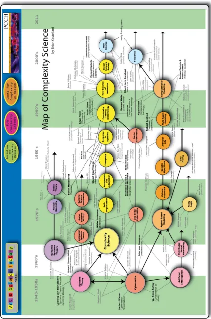
of organisms. We illustrate this plurality of settings by an image from “Arts and Science

Factory”, see figure 1.1.

Current Understanding As complexity science gained footing, so too did the philo-sophical speculations return. The semantic distinction that has been applied most in the

recent years is that between strong and weak emergence. The term weak was coined by

Mark Bedau in an effort to find an appropriate operational definition to a concept already

in use. In Bedau [1997] the description is that of behaviour resulting in a macrostate that is

derivable only by simulations from the dynamical and the external (and initial) condition4_.

3_{This entropy of a stochastic process is fundamentally different to the entropy introduced by Kolmogorov}

and Sinai as a function of measurable dynamical systems.

(16)

[image:16.595.109.537.70.717.2]

(17)

In Paul Davies and Niels H. Gregersen (editors) [2010] the editors observe that our

con-ceptions of reality readily model themselves on the latest technological advances. Bedau’s

definition appears to fit the same trend - recent scientific progress relied heavily on the

new-found ability to simulate behaviour. Consequently weak emergence views reality through

this particular prism.

These are metaphysically noncommittal, scientifically comfortable stances. One does

not need to reject the monoistic structure to admit unpredictability: the simple fact that

equations are not analytically solvable means that there is a limit to how much can be

forecast. There is thus a distinction between predictability in principle and in practice.

A lot of the theoretically deducible phenomena can thus be called emergent. The prime

examples here are deterministic cellular automata (Games of Life), behaviour of networks,

or various aspects of evolution. Thus this description does not single out outcomes based

on whether they are in any way interesting or surprising; but rather by indicating systems

that we cannot (yet?) solve, it seems to have an operational-based support: most emergent

macro phenomena are discovered only with the use of simulation. However, we do not know

that in some years’ time there won’t be a new mathematics capable of giving the analytic

result. Thus Grelling (as mentioned in Hempel and Oppenheim [1948]) points out that this

view of weak emergence is more of a provisional construct.

In this respect it is half way to the more safe approach of doing complexity science without

taking a metaphysical stance. From Thor´en and Gerlee [2010]: “Contemporary accounts

typically strive for weaker formulations trying to salvage some part of the concept whilst

giving others up”. Chalmers [2006] gives a slightly different definition. Here weak

emer-gence concerns truths that are unexpected (in contrast Chalmers’ strong emeremer-gence is about

truths that are not deducible). Thus too deterministic cellular automata are weakly

emer-gent - even if one would need to resort to calculations the general behaviour could still

be deduced. Weak emergence becomes more of a statement of our understanding of the

propagation of causality; giving our epistemological position relative to that of Laplace’s

demon.

Chalmers is also careful to mention that in general weak emergence should say something

about the level of difficulty with which the inference takes place, as well as the difference

between the complexity of the combination rules and the overall behaviour. The

(18)

achieved by including all the aspects desired intuitively. A phenomenon is weakly emergent

if complex, interesting high-level function is produced as a result of combining simple

low-level mechanism in simple ways. (Ibid.)

Strong emergence, on the other hand, tends to place itself in direct opposition to

reduc-tionism5_{. Accepting this hypothesis means allowing for the existence of laws other than}

the ones inferable from the scientific methodology, which in turn essentially involves a new

kind of science. Here once again there are different schools based on what assumptions or

consequences the authors are comfortable with ascribing to this concept. Thus for example

Davies [2004] attributes to emergents novel causal powers, and admits downward causation,

typically a problematic concept for scientists, one that is most required to be taken on faith.

Kim [2006], on the other hand, suggests that philosophical coherence makes it not as simple

as just picking attribute - and that admitting some may lead to undermining the whole

concept, which is what happens with the circularity of downward causation6_.

Strong emergence is a philosophical conjecture, which for example for Kim [1999] should

con-tain both irreducibility and supervenience. Starting from that approach the main question

becomes whether strongly emergent phenomena exist, and if so, what they are. Chalmers

supports the view that consciousness is exactly that. Depending on one’s theological

lean-ings God could also be ‘analysed’ in this way (Peacocke [2010], Gregersen [2010]). Though

of course since the answers depend on the definition the results are possibly incomparable.

We will be attempting to quantitatively describe the extent to which initial

infor-mation persists across in time. We too will use the distinction between the strong and

weak notion in the loosest possible sense, focusing on epistemology rather than ontology

even in the ‘strong’ case. That part of the thesis that refers back to it does so not because

it claims to have found a phenomenon that we claim to be strongly emergent, but rather

to notice that a certain statistical function can be used to differentiate between the two

conceptsgiven they are defined in a certain way. The data used is from chaotic dynamical

systems, but our function sees chaosas such as a completely uninteresting (giving nothing

in terms of forecastability) background noise, looking instead for global structures. The

crucial conceptual link between low-dimensional dynamical systems and high-level complex

5_{Everyday usage had a diluting effect on the notion of ‘strong’. If ‘very strong’ (Clayton [2006]) is already}

in literature, the next step is naturally some form of scale. Bauchau [2006] tentatively proposes one that places chaos somewhere low down, the top being defined by the class of universal computation.

6_{Chalmers also talks about downward causation as a phenomenon in its own right, not necessarily}

(19)

systems can be drawn in a number of ways, defining the ‘higher’ level at an arbitrary,

sub-jective degree of complexity. One such is to consider the trajectory as a ‘complex’ object,

which can be characterised by some aggregate variables e.g. the Lyapunov exponent

-but comes about as a result of, simply, applying the map. Alternatively the dynamical

system itself, with the related quantities characterising the geometry, say, of the underlying

strange attractors, can be thought of as an ‘aggregate’, whose succint properties can best

be understood not by looking at the equation, but indeed by the aforementioned variables.

In the next section we will see that according to our definition of emergence, a chaotic

attractor with no interesting structure would not be considered as giving rise to emergent

(20)

1.2 The Probabilistic Framework

We now review a common language in which various correlation, complexity and emergence

measures are typically expressed.

The usual aim of physical sciences is to establish a link between observations and

reality via an idealisation (a model). The distinction is that reality results in our

observa-tions that, in turn, lead to statements about the idealisation. Logic builds a reverse link

and allows predictions from the model to be tested against new observations. Consider an

archetypal process of tossing a fair coin. Without making a statement about reality we can

successfully model the process by random variables. The key word here is ‘successfully’,

which means that there do exist functions of results that are predictable by the model.

Development of probability theory can be traced in the correspondence of Pascal and

Fer-mat, established after Pascal’s friend Chevalier De M´er´e brought to his attention the issues

facing gamblers at dice; especially the Autumn 1654 series. Along with establishing the

basic rules of the calculus of probabilities, Pascal introduces probability as a value between

0 and 1 that is in some way “attached” to an event (rather than being dependent on the

mind of the observer, as M. Miton (see Renyi [1972]) would have it). It expresses the extent

of certainty that the event will happen, which Pascal identifies with the actual likelihood of

an event coming to pass. The term “probability” is chosen especially so that its numerical

value corresponds to our intuitive conceptual use of it7_.

Pascal also suggests that measuring the probability is equivalent to observing relative

fre-quencies of occurrences in long trials. Probability is thus a fixed value around which the

relative frequency oscillates in a random fashion. This leads to an effective two-level

ran-domness - uncertainty in how sure one is in an event happening.

This put a start to both the mathematical and the scientific discipline. Probability can be

approximated by observations, and subsequent manipulations using the calculus of

prob-abilities allow for prediction, at least statistically. Pascal stresses that partial knowledge

about the likelihood of an event occurring or not still constitutes some kind of knowledge

about the event, even though the event might not actually come to pass.

7_{Nowadays Pascal would have even less reason to worry that the meaning of “probable” - as a theological}

(21)

That these statements can be made scientifically rigorous8_{, and can be put on a}

firm mathematical basis, has been postulated only relatively recently. It was Doob and

Kolmogorov that proved that the rules of chance constitute a mathematical framework

-see Getoor [2009] for a review.

We state the formal probability framework. Let (Ω,F,P) be a probability space,

and (E,E) a measurable space. We interpret Ω as the space of all possible realisations of

the given process. The σ-algebra F on Ω is then the respective event space, and P is the

probability measure. We take E to be a subset of Rn for some integer n, and associate it

with a measurablestate space of the system.

A motivation in separating Ω from E, the space of possibilities from the potential results of measurements, can be traced to the wish to be more exact about the meaning of

mea-surement. Consider performing any experiment, by which we mean some interaction with a

system. It is more usual to measure some feature of the system. In this case it is more

obvi-ous that the result of the measurement would be a function of theactualstate, X: Ω_→E. Measuring the temperature of gas in a box falls in this category9_.

Our observations thus fall in E. Let e _∈ E. Since we identify what we observe with a function of the state of the system,

e=X(ω), (1.1)

whereω_∈Ω is the state of the system. We call functionX a random variable, or a variate, or chance variable.

1.2.1 The Concept of Probability

Suppose we take the frequentist approach of associating the likelihood of seeing an outcome

with the relative frequency with which this outcome has already been observed in systems

of this kind. In this approach relative frequency serves the purpose of creating a measure

on E. A random variable was setup as a link between observations in E and some “true” states in Ω. So the probability of seeing e_∈ E can be thought of as resulting from some probability of the system being in those states that lead to observinge. Hence the common definition of probability: given a random variableX, the probability of observing it take a

8_{ignoring the ‘truth’ contained in them for a moment - see Diaconis et al. [2007]}

9_{We make the optimistic assumption that there is a correspondence between reality and state of the}

(22)

valueA⊆E,

P(A) =P(X_∈A) =_P{ω _∈R:X(ω)∈A}. (1.2)

In information theory/computation mechanics literature the sets Ω and E are often identi-fied with each other, and the random variables that question the state become the identity

functions (although most of the time Ω is not being considered at all).

1.2.2 Entropy and Entropic Concepts

Entropy was introduced as an experimentally determinable quantity expressing the way a

system absorbs heat at a given temperature. It was associated with the lack of organisation

or order. The second law of thermodynamics posited that in a closed system entropy

increases. Boltzmann attempted to justify the second law by replacing the imperative

with, simply, vast differences on the scale of improbable. In his framework thermodynamic

entropy measured the number of possible configurations of constituent parts that made up

some distinct observable state.

Let X : Ω_→ E be a random variable, andP defined by 1.2. The Shannon information of discrete-valued random variable X, introduced in Shannon [1948]10 _is

H(X) =−X

x∈E

P(x) logP(x). (1.3)

In a countably infinite support space entropy is defined only if the series converges.

We will also use the differential Shannon entropy defined when p(x), x _∈E is probability distribution, and given by

H[p] =−

Z

x∈E

dx p(x) logp(x) (1.4)

but we will mention the difference between the two later in the text, in a particular context.

Whatever information and uncertainty are, conceptually uncertainty is often understood to

be the absence of information, and vice versa. Consider a random variable. Before

obser-vation there is some uncertainty as to the outcome. Obserobser-vation corresponds to obtaining

an amount−logP(x) of information. Thus entropy is defined as the average information of a message. Note that even information content in a message doesn’t depend on the specific

10_{The probability} _P _{is understood to be given; the implication is that the variable is associated with}

(23)

message itself, but rather on its probability, a property conferred on it by the system (or

by the observer’s knowledge of the system). Thus entropy is a function of the measure P

and not of the support space.

Relative and Conditional Entropies Given two random variables X and Y,

X, Y : Ω_→E we define the joint entropy

H(X, Y) =₋ X x,y∈E

P(x, y) logP(x, y), (1.5)

whereP(x, y) is the joint probability. The conditional entropy is then

H(X|Y) =H(X, Y)−H(Y). (1.6)

Conditional entropy measures the amount of uncertainty in the outcome of one variable

(hereX) given that the outcome of another (Y) is known. Here we always useP to express the notion of probability. The way we defined it earlier rests on the assumption that each

random variable comes with a probability we tacitly understand to be its own. ThusP(x) is actually equal to the measure PX{X−1(x)}, and P(y) isPY{Y−1(y)}, wherePX and PY

are for example given by the relative frequencies of the variables and are not necessarily the

same. Thus P stands for a loose sense of ‘probability of a random variable’.

The form 1.6 is the functional form of a ‘distance’ in the space of measures: if LetP, P0 _be measures on the space of measurable outcomes, then the relative entropy, or the

Kullback-Leibler (KL) divergence betweenP and P0_{, is defined to be}

KL(P_||P0) =X x∈E

P(x) log P(x)

P0₍_x₎. (1.7)

Here we separate P from P0 _{because we view them in their capacities as probability} mea-sures.

The logarithm is defined to be equal to zero whenever P0₍_x_{) = 0 or} _P₍_x_{) = 0. KL is not} symmetric, and is not technically a metric. Also 1.6 is not symmetric - the information

(24)

Mutual Information The mutual information (MI) betweenX andY is

I(X, Y) =H(X) +H(Y)−H(X, Y). (1.8)

As entropy is extensive, the sum of entropies of independent variables should be the same

as the entropy of the system made up of these variables. If the joint entropy is less than

the sum of marginals it is understood that reduction in uncertainty is at the expense of

some interdependence. Mutual information measures the deficit, and thus the degree of

interdependence between two variables. It is zero if the two variables are independent (since

the joint measure becomes the product of the marginals), is also completely symmetric and

always positive.

MI can also be written as

I(X, Y) =H(Y)₋H(Y_|X). (1.9)

This form expresses MI as the difference between uncertainty in one outcome (hereY) and the uncertainty in that outcome given that we know the result of another outcome (X). It is thus the information about one variable stored in the other, and is, too, symmetric11_.

Writing MI in terms of probabilities,

I(X, Y) = X x,y∈E

P(x, y) log P(x, y)

P(x)P(y), (1.10)

we see that mutual information between two variables is actually the relative entropy

be-tween the joint distribution and the product of the marginals. If the two variables are

independent the jointbecomes equal to the product of the marginals, and so the divergence

between two elements that are actually the same point is zero (here the support space is

actuallyExE).

1.2.3 Stochastic Processes: adding time

The framework into which this brings us is that of stochastic processes, i.e. systems where

predictability of evolution can be treated using probabilistic tools. A stochastic process is

11_{The information-theoretic framework lends itself to verbal abstractions of the intensity limited only by}

(25)

defined as a sequence of random variables:

{Xt, t∈T}. (1.11)

Some care must be taken when introducing time. The mathematical framework for discrete

processes, otherwise known as sequences, (T = Z) was established by Kolmogorov, and

Doob did the same forT =Rwhich presented more difficulties.

There are several ways of expressing the random variables. Behind the ideas are

essentially three spaces: outcomes Ω, statesE and time setT. X(ω) is the random variable independent of time. Including it produces X(ω, t), or Xt(ω), the latter notation being more common in the discrete time case.

The strength of this framework is that it allows to formulate dependencies between

variables, which in this case are states at different times. It is a language of choice for

models where evolution is probabilistic.

The mathematical object encoding any apparent causal structure between states at times

in some set T is the joint probability of events indexed by elements ofT.

Suppose that we have a discrete clock (which we take to be represented by Z) that

ticks from_−∞to_∞, and that at every given timei_∈Za system yields a value from some

alphabet A. Thus a specific bi-infinite run of the system gives us a sequence (an element

of space AZ). We want to consider a random variable connected to a fixed time i, or more

generally to a block of times from a to b. We can construct a probability space (Ω,F,P),

where Ω =E =AZ,Fis aσ-algebra of cylinder sets, andP is a probability measure of Ω.

These random variables can be thought of as blocks, or subsequences. The above

con-struct allows us to talk about probability over blocks of arbitrary length. Let Sb a =

(Sa, Sa+1, ..Sb), b, a ∈ Z, b≥a be a block of length b −a+ 1 s.t. Sa := Saa; and let →

Sa to be the semi-infinite block starting at a,S→a= (Sa, Sa+1, Sa+2..), and

←

Sa = (..Sa−2, Sa−1)

to be one ending at and not inclusive of a. We define a stationary process as one whose marginals depend only on the length of the subsequence. No major global changes occur in

such processes, changes that influence the relative frequency of subprocesses. Stationarity

is defined as system with

P Sa+N a =A

=PS_bb+N =A, (1.12)

(26)

N, which we call SN_{, N} _∈

Z+.

Entropy Rate and related quantities

Consider the the uncertainty inherent in the system. A way of quantifying the amount

(rather than perhaps the role) of chance is to view the data as an outcome of a stochastic

process detailed above, and enquire after the entropy per symbol, where by symbol we mean

an element of the alphabetA. This quantity is also called the entropy rate. We follow the

methodology established in Shannon [1948] and define Shannon entropy per block of length

N,HN, as

HN =H

SN:=− X

A∈_AN

P(SN =A) logP(SN =A). (1.13)

The block entropy is always nonnegative,HN ≥0, and grows monotonically withN,HN0 ≥

HN,∀N0 > N, N, N0 ∈Z+. Shannon defines two quantities, the entropy per symbol in a

block of N random variables (starting at zero),

GN :=− 1

NH[S

N−1

0 ], (1.14)

and the average entropy of a new symbol given some past,

FN :=−H[S1 |S0−N+1], (1.15)

This is a function of random variables related to each other by the relative time of

occur-rence, so that the index of the block beginning is by itself arbitrary and is here shown as

zero by default (see Cover and Thomas [2006]).

For stationary processes the limits for both GN and FN as N → ∞ exist and coincide (Shannon [1948]). Hence the definition of the entropy rate h of a stochastic process S

(considering thatGN is of course just the normalised block entropy):

h= lim N→∞−

1

NHN. (1.16)

To illustrate features h picks up on consider:

(27)

become independent and hence

h= lim N→∞

1

N

N X

i=0

H[Si].

Here existence of h is assured unless H is a function of i, which is of course the blueprint of non-stationarity.

• Si are independent and identically distributed (i.i.d.), then

h=H[S0],

where the index is again arbitrary. The average entropy per symbol isthe entropy of

a symbol, since all symbols have the same uncertainty. This is not usually true, as

h is a property of the system as a whole, a function of the information source rather than of the outcome at some single point in time. That the two are the same here

shows that the information source does not store time dependencies.

• If, additionally, each i.i.d. Si has a uniform measure of a support space of cardinality

M,H[Si] = logM, and hence

h= logM.

Thus for a coin toss modelled as a stochastic process with i.i.d. outcomes the alphabet

would consist of two entries, giving the entropy rate of log 2.

Any skewness in the measure towards a particular outcome of any variate would

decrease the entropy rate of the process. Any dependency between variables would reduce

the uncertainty per symbol and hence decrease the entropy rate even further. h measures both effects. As we have seen above, it is maximal for i.i.d. variates with uniform measure.

1.2.4 Symbolic Dynamics: linking Deterministic and Stochastic Frame-works

Consider a mapF :X _→X and a partitionP on the state spaceX=F_i_∈_CXi,PM :X →

{1,2, .., M}, where Fstands for the disjoint union.

(28)

for convenience we here label with the same letter, turns each orbitO

O= x, F(x), F2(x), .. (1.17)

into a symbolic orbit sequence:

PM :O→ΣF (1.18)

(x, F(x), .. )_7→(PM(x), PM(F(x))..), (1.19)

where Ois the set of all orbits. Thus ΣF is the set of all possible, or admissible, symbolic

orbit sequences associated with the partition PM of X, and map F. Note that orbits are defined as being bi-infinite: s= (st)∞t=−∞. Orbit sequences are thus sequences of integers labeling the position of the orbit in the coarse-grained version of the state space.

The symbolic dynamical system is defined as (ΣF, σ), where the subshiftσ is equivalent to the evolution operator, mapping each symbol to the next one (and is as such a function of

the entire sequence itself, rather than the symbols):

σ: ΣF →ΣF (1.20)

σ(PM(x), PM(F(x))..)7→σ(PM(F(x)), PM(F(F(x)))..). (1.21)

This shows the process by which one can contextualise the study of dynamical systems in

(29)

1.3 Toy Models

1.3.1 The Logistic Map

The initial motivation was a model describing population growth. It is clear that in order

to allow for some form of stability the system would have to be nonlinear. Interestingly

enough, applying the same arguments behind parameters and form of dependencies to

a continuous version produces a rather straightforward and unsurprising result, one that

certainly does not admit chaos: one-dimensional iterative maps can exhibit a much broader

range of behaviour then the corresponding one-dimensional ODE. Yet the map is only one

of the possible ways to discretise the logistic equation, some of which produce quite different

results. Behavioural richness of this particular version, the logistic map, was first noted in

May [1976].

The logistic map f is a one-dimensional dissipative system displaying the period-doubling route to chaos. For 0_≤r _≤4,f : [0,1]_→[0,1], and for r >4 the trajectories are no longer confined. Ifxn+1 =f(xn),

xn+1=rxn(1−xn). (1.22)

For small r the motion is periodic. With increased r the periodicity successively doubles until what is known as the period-doubling accumulation point at rc<4. The underly-ing pitchfork bifurcation produces unstable periodic points, makunderly-ing the attractor at rc be nowhere dense. It can be shown that then the attractor is a Cantor set, with a variety of

computable fractal dimensions (see for instance Grassberger and Procaccia [1983a],

Grass-berger and Procaccia [1983b]). At 4 > r > rc motion is confined to chaotic bands. These then merge in a symmetric way until atr= 4 the attractor fills [0,1] and motion is mixing, in the terminology of Collet and Eckmann.

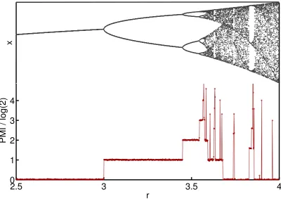
Figure 1.2 shows the bifurcation diagram. On this scale it would not matter if it was

produced by following single trajectories, or taking a number of certain initial conditions

and recording the iterates at a specified time. The only persistent feature of the map is the

clock. Chaotic motion conforms to this by making everyTth _{iterate be located in the same} band (ifT is the number of bands), but leaves the location of the point within the band to be varied with a certain positive Lyapunov exponentλ(r). Lorenz called this motion ‘noisy periodicity’.

Figure 1.3 shows the variation of the Lyapunov exponent (of which there is only

(30)

[image:30.595.152.494.104.363.2]

Figure 1.2: The standard bifurcation diagram of the logistic map. For lower values ofr the trend continues, the attractor x having a periodicty one (source: wikipedia).

[image:30.595.162.488.452.687.2]

(31)

to windows of regular motion. On the bifurcation diagram these are regions with distinct

lines. The biggest window is around r = 1 +√8, where the attractor is a period-3 limit cycle. These bursts of periodicity happen at all scales of rc < r < 4. Moreover, they do not necessarily then lead to chaos in the same way. Period-tripling, and other combinations

and mergers can be detected if only the r resolution is large enough.

The logistic map lies in the broad class of one-dimensional unimodal maps which

all share the qualitative features of the bifurcation pattern (to be more precise, through

kneading theory they can be shown to be topologically equivalent). These maps are

pro-jections of higher-dimensional systems to lower planes, and as such are not invertible (for

example through having several of higher-dimensional orbits happening to have an equal

coordinate). One of the reasons behind their generality is that often the dynamics of these

original systems happens only on a small subset of the state space, and as such motion

can effectively be described by simpler lower-dimensional maps. The general theory of 1D

maps is limited: it is for instance not possible to find all ranges of (to use our example)

r corresponding to motion of a particular type. Something similar is possible in reverse (Singer [1978]): satisfaction of a certain condition on the Schwarzian derivative (a function

of the derivates of various orders) can demonstrate a limit on the number of stable periodic

orbits. The opposite means the attractor is either infinite (a cantor set), or motion is mixing

with all the traits of chaos. In this respect the logistic maps belongs to the class of maps

with an everywhere-negative Schwarzian derivate, labelled S-maps.

The existing general result concerns the types of motion possible, and is in fact the reason

the logistic map displays both mixing, periodic and ‘ergodic’ (infinite attractor) behaviour.

It is that subsets of r that result in these three motion types are all of positive Lesbe-gue measures. Another interesting result is the Sarkovskii sequence, which says that if an

observed period is present in the given sequence, then the system also has motion with

ar-bitrarily long periods. The lowest periodicity in the sequence is three, which is exactly the

value mentioned above for the logistic map. This result also proves that an infinite range

of other periodicities can indeed be detected. In fact since for low values of r the period doubles, it implies that the periodic windows (which do not have to have period equal to

2n_{) can be infinite in number. That is indeed the case. In fact the sequence does not limit}

the number of windows with the same period.

(32)

systems defined by flip bifurcations. Periodicity doubles every ri, leaving behind unstable fixed points, so that if

δi=

ri−ri+1

ri+1−rr+2

(1.23)

then the Feigenbaum constant δ∞ = 4.6692 defines a certain class of maps. Another way chaos sets in is through intermittency. This is a direct effect of the tangent bifurcations

that are the underlying reasons behind the attractor suddenly turning periodic. This

pro-cess leaves trajectories for some finite time stuck near specific points. This is the effect that

makes us see the pattern of folded shadows in the bifurcation diagram: these specific regions

are exactly ones which, after a small increase in r, become the stable periodic limit cycles. Inside these periodic windows after periodicity increases (in a manner that is not necessarily

doubling the period) noisy periodicity occurs again, until an ‘explosion’ happens. This - or

the ‘interior crisis’ coined by Grebogi - is the sudden jump in the size of the attractor.

At r= 4 under a change of variables the motion is equivalent to the Bernoulli shift map (bit shift map) (and also to the behaviour of the Tent map atµ= 2, see later section), given by

xn+1= 2xn mod [1] (1.24)

If we representx in binary form then points are sequences composed of two symbols. Itera-tions can then be viewed as shifting the sequence (which is to the right of the decimal point)

one step to the left. One of the ways in which this shift in framework is useful is in how it

helps to understand the effects of chaos, represented in the logistic map by mixing motion.

Chaos is often characterised by sensitive dependence on initial condition. In practice this

means thatfinite information about an initial condition will soon be lost. Any finite

infor-mation is represented by a finite binary string. Hence after the number of iterations becomes

greater than the length of the initial string no information about the original string would

be left. More exactly, if two trajectories differ by some finitely-specified amount, there is a

time after which this difference would be nullified12_.

This is one the reasons we use chaotic dynamical systems in our study of how information

gets preserved across time. We do not view chaos asthe emergent phenomenon; we are only

partially interested in its phenomenology. From the perspective of this work chaotic motion

12_{Initial conditions that are rational numbers would thus be repeated ever finite number of steps, since}

(33)

merely serves as a mechanism that after a finite time makes computing the true final state

impossible. Note, however, that that does not mean that we cannot say anything about

where trajectories are likely to end up. The invariant measure is a beta function and is

not flat. That means that independent of the initial condition there are guesses about the

position at some arbitrarily far future, guesses which are more likely to be correct than not

(for same subset size). Accordingly, in our investigations we focus not on prediction but on

‘forecastability’ (the difference is clarified in the section on PMI).

As such the interesting features we find stem from other persistent features of the system,

or from a variety of motion, not just chaotic; or else from the different ways in which chaotic

motion can happen. The latter two are explored by a different system which we give in the

section below. Unlike the logistic map it is not dissipative but rather admits coexistence of

various types of trajectories, exhibiting a different route to chaos and is thus accompanied

by a range of new phenomena.

1.3.2 The Standard Map

The standard map, also sometimes called the Chirikov standard map, was considered by

Bryan Taylor, and introduced by Boris Chirikov in Chirikov [1979]. A two-dimensional

area-preserving map with a single parameter, it is a Poincar´e cross-section of a

Hamilto-nian system that demonstrates the now-classic route to the onset of chaos described by the

KAM framework. As such it has been found useful in such a wide variety of situations (see

Zaslavsky [2012]) that its common name has come to reflect its applicability. The classical

interpretation of the associated Hamiltonian system is that of a kicked rotor. The quantum

version of the Hamiltonian behind the map is used to test the Anderson Localisation.

The map is paradigmatical in its demonstration of Hamiltonian chaos (according to Cambell

[1987], it plays the same role for Hamiltonian chaos the logistic map did for chaos in

dissi-pative systems). What makes this map so tractable as a toy model is that there is only one

parameter that essentially controls the system regime. The fact that the map is iterative

also means computations can be performed relatively fast, with potential errors stemming

(34)

The standard map is given by

pn+1=pn+Ksinθn (1.25)

θn+1=θn+pn+1. (1.26)

Without loss of generality we takeK to be positive, and since here we will be considering the dynamics on a torus, both variables are confined to the fundamental domain [0,2π], and taken mod [2π]. A negative K corresponds to a translation of angle to [₋π, π], and graphically it merely shifts the position of the main structure surrounding the stable fixed

point. The map is reversible and has a number of symmetries.

The extent of chaos increases with K, so that at K = 0 all the orbits are either periodic or quasi-periodic, and at K = 2π the system is ergodic, at least on the level of available resolutions (finding the measure of these islands of regular motion for large K is one the open problems - see Sinai [2010]). We will restrict our interest to 0≤K ≤2π.

The original Hamiltonian for the kicked rotor, with kicks of strength K, is

H(θ, p) = 1 2p

2₊_K_cos_θ

∞ X

n=−∞

δ

t T −n

, (1.27)

where p is the canonical momentum, and δ represents instantaneous kicks at frequency 2π/T. It is clear that whileθ is continuous throughout,pgets changed by a finite amount. Therefore one can look at the Poincar´e plane defined by the tjust before successive kicks. These difference equations are equivalent to the standard map, and can be derived from

Hamilton’s equations associated with eq.(1.27)

In this respect the state space of the standard map can be interpreted as the phase space

of the Hamiltonian, and momentumpand angleθas polar coordinates of the trajectory as it goes through the Poincar´e plane.

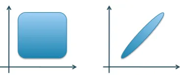
The range of map behaviour is demonstrated in figure 1.4 that traces the evolution

of a number of trajectories for three different K. Broadly speaking, circles correspond to regular orbits and absence of structure indicates chaos. These graphs show one of the more

striking (Zaslavsky [2012]) features of Hamiltonian chaos - the coexistence of regions of

regular and chaotic motion.

(35)

(a)K= 0.6 (b) K= 1.1 (c)K= 2

Figure 1.4: Evolution of a number of trajectories using the standard map with increasingK

(here the axes are (θ, p), ₋π _≤θ_≤π). Orbits are tagged by colour. Notice that atK = 2 no single area (apart from maybe near the resonances) is dominated by a single trajectory. This is not the case at K = 1.1, where for large enough times trajectories are still seen to stick in subsets of the broad chaotic area. See figure 1.5 for more of this effect.

attractors. The volume (say the set of trajectories) does not contract to a small subset of

the initial state space. Hamiltonian systems by definition conserve energy, or the phase space

volume, which in terms of the standard map translates to area-preservation. Varying K

therefore changes the general type and the specifics of motion given by an initial conditions.

Thus the absence of kicks modelled by strength K = 0 renders the original Hamiltonian integrable. Just by looking at the equations shows that this is because momentum is now

a conserved quantity (along with energy). If θ had not been confined the system would simply be describing free motion. As it stands the invariant manifolds are described by

circles, each defined by a winding number ω(p0) =p0:

pn+1 =p0 (1.28)

θn+1 =θ0+p0n. (1.29)

This regular motion, which involves trajectories confined to horizontal lines on the phase

diagram, comes in two types. If ω is rational then after a finite number of iterations the trajectory begins to retrace its steps. Thus in periodic motion for some initial angle the

horizontal lines fill in to a greater extent (with smaller gaps) depending on the specifics of

ω. They do so without any gaps, densely covering the circle, ifωis irrational, in which case the motion is quasi-periodic. Hence (0,0) is a fixed point, every point on the ω = π is a period-2 fixed point, etc.

(36)

is no longer equal to p0. For example atω = π theθ = 0 and θ= π are now stable fixed

points between which lie hyperbolic fixed points. Point stability can be tested by

compar-ing the trace of the Jacobian to 2 in order to compute Greene’s residue. The stable fixed

points become surrounded by elliptic orbits, and the hyperbolic fixed points are associated

to hyperbolic orbits and thin stochastic bands. All these have an associated periodicity so

that ellipses around the period-two fixed points are populated by trajectories alternating

between them at every time step. Thus the horizonal frequency of these elliptic islands can

easily be predicted. These ellipses come in what can be described as ‘islands’, or resonances.

Circles associated with periodic motion - rationalω - typically break down first, atK = 0. According to the Poincar´e-Birkhoff theorem for every ω = m/n there will be at least two periodic orbits left, with periodn(Meiss [2005]). This appears asnislands, the chain called a resonance. At least one of those will be on the p= 0 line, the ‘dominant’ symmetry line (ibid.). As K increases new elliptic orbits are created around each elliptic orbit based on the associated ω. Thus structures form on all scales, though this is still not proven. In terms of universality, MacKay [1983] used renormalisation group techniques to show that

the island structure around the golden curve is the same for all smooth maps (twist maps).

The arrangement of islands of periodic motion is non-trivial. A single chaotic orbit will

encounter obstacles on all scales, which corresponds to there being a specific distribution

of island sizes. The area occupied by a single chaotic orbit will be finite (Umberger and

Farmer [1985]), turning the orbit into a ‘fat fractal’. If it is computed by for example

breaking up the state space and counting the visited squares then this number will have

definite scaling regime with resolution. The reverse holds too and the regular motion also

occupies a finite area (Cambell [1987]). GrowingKis generally associated with deformation of the horizonal lines, or rotational circles (the circles seen as circles in the state space do

not actually encircle a torus, and are called librational circles). As these encroach on each

others’ spaces the stable manifold of one crosses the unstable manifold of the other in a

‘resonance overlap’. This produces a homoclinic intersection, and therefore an infinity of

homoclinic intersections. Partially motivated by the study of motion in plasma, Chirikov

[1960] computed the criteria for the overlap of the resonances. If the state space is viewed

as a cylinder then the destruction of the final barrier allows the ‘particle’ to escape, i.e.

momentum to increase indefinitely. This gives an estimate of someK =Kc.

It is possible to determine existence of a rotational circle by looking at convergence of

(37)

Thus with increase in K fewer and fewer circles are left. This relationship between the winding number associated with the remaining circle and the K value can be made exact. Works such as Black and Satija [1989] show the ‘fractal’ nature of this dependency. The

last circles to be destroyed correspond to ones withω =γ_±m, m_∈Z, whereγ is the ‘most’

irrational (the criteria assigning the extent of ‘irrationality’ is related to the asymptotic tails

in the fraction expansion) number, the golden mean. MacKay and Percival [1985] proved

that no circles are left forK >63/64. We use the notation Kg to denote the exact point of the breakdown of the golden circle. Although no analytic expression exists, numerically it

is found to be K≈0.97. Kc≥Kg, and the two values are usually associated.

All the above is usually phrased in terms of flows in the state space of the original

Hamil-tonian, so that invariant circles are cross-sections of the invariant tori, called the KAM

(Kolmogorov-Arnold-Moser) tori. The KAM theorem is then exactly the statement about

persistence and breakdown conditions of these KAM tori (and hence cantori). Also in this

frameworkK can be viewed as perturbation away from integrability, in at least one meaning of the word.

Transport in the Standard map Stochastic motion occurs between the invariant ro-tational circles. A region that is bordered by them and containing nothing inside to limit

the chaotic motion is called a ‘zone of stability’. Mather [1991] showed the existence of

orbits that get asymptotically close to the regions’ borders. These regions may be difficult

to pinpoint whenK≈Kcsince then the structures are self-similar and appear on all scales. According to the Aubry-Mather theory irrational winding numbers are associated with

tra-jectories dense on either the circle or a Cantor set. Since the circles stop existing after some

finite K, it follows that what remains must become a cantor set. These ‘cantori’ will thus contain holes which then admit movement to the other side, and chaotic trajectories can

pass through.

Figure 1.5 shows the consequence of this method of freeing up the space. Since

passing through the obstacles that are cantori is difficult, there are time scales (possibly

location-dependent) at which trajectories are essentially stuck in specific regions. While

there they mimic the rotational motion that characterised those regions before the circle

(38)

(a)t1 (b)t2 > t1 (c)t3 > t2

Figure 1.5: The same run of the standard map showing the evolution of trajectories at

K = 0.971635 up to someti. As before a trajectory has its own colour, and the colour of a pixel is determined by the same orbit sequence across all pixels. Therefore if there are two areas that change in colour, but are at some time coloured differently with no mixing, it means that there is a time period in which at least one signed trajectories isnot entering a particular subset.

Notice how occupation of the different areas of the graph fluctuates, the most uniformly colour areas being near the separatrices - and the distinct change in colour of the two bands that appear to be symmetric about the golden circle, which lies roughly in the middle.

can be written as

∆W ∝(K−Kc)a, (1.30)

a≈3. This is roughly in line with the prediction in Chirikov [1979] expressed in terms of

time of transitions between regions. These results can be expressed in terms of the

diffu-sion coefficient, calculated using the Fokker-Planck framework in which it makes sense to

consider passing through a barrier as a probabilistic phenomenon.

A global picture with analysis integrating diffusion across the different trajectories suggests

anomalously slow relaxation due to the cantori. Poincar´e recurrences (Chirikov and

She-pelyansky [1999]) and for instance the number of trapped particles in a region then decay

(39)

1.4 Quantifying Complexity

The existing measures of complexity and emergence all vary depending on the

mathemati-cal framework one considers, the system in question, and of course on what one’s intuitive

notions about the extent of ‘emergence’ in this system are. Broadly speaking there are

measures based on single realisations and multiple realisation, or ensembles. To the former

category belongs the algorithmic Kolmogorov complexity (see below). We hold the view

that randomness should not be equated with complexity or emergence, and so our proposed

measure is a function of probabilities. As seen above, in that setting the order-disorder

relation is usually phrased in terms of entropies, which is exactly our aim.

The measure in existing literature to which our function comes closest is Effective Measure

Complexity (EMC, otherwise known as the excess entropy). This quantity is usually

con-ceptually twinned with the entropy rate, in the sense that defining one can define the other,

and certainly understanding one helps with having a clear picture of the other. Entropy

rate was already introduced in eq. (1.16) in the context of sequences. Thus EMC and

entropy rate are measures of systems with a discrete alphabet (and by extension discrete

time). Excess entropy is usually applied to sequences obtained from symbolic dynamics or

probabilistic cellular automata, whereas the EMC incarnation (the original) was studied in

formal languages and grammar.

Symbolic dynamics then looks at the map as a potential means of randomisation. The same

notions can be defined in terms of continuous state spaces to obtain metric entropy and its

measure-free counterpart, topological entropy. These are standard quantifiers in dynamical

systems theory.

In our work we use data from dynamical systems without any discretisation. There is still

a notion of resolution, but that is now related to the depth of sampling, and is therefore

phrased in terms of varying the measures of subsets rather than their linear size. Our initial

aim is to test a function that could detect shared information between the past and future

of a distribution over the attractor, with a variable time gap, and understand what features

of the system would qualify it for being labelled, in this definition, as ‘strongly emergent’.

In the following section we set the mathematical context of the various quantifiers of

order and disorder mentioned above, and then review the toy models that we will use. These

(40)

[image:40.595.232.416.94.204.2]

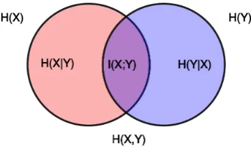
Figure 1.6: Venn diagram where the extent of overlap of two variables measures the degree of their interdependence on each other, in other words their Mutual Information (denoted here by I(X;Y). H(X, Y) is the joint entropy of X and Y. Source: wikipedia.) Some systems that we will study have the constant marginal entropies, which means that looking at the cross-section is equivalent to looking at the joint entropy of the system.

map, a two-dimensional area-preserving map. Both are maps with one-parameter, changing

which affects the extent of chaos in the trajectories. Chaos is a standard setting in which

to talk about ‘weak’ emergence. In general in dynamical systems attractors are sometime

said to ‘emerge’ as parameters are varied. We view chaos as a mechanism that results in

the loss of initial information. In the language of dynamical systems that is described (and

defined) by the rate of exponential divergence of nearby trajectories, and the quantity that

measures it is related to the metric entropy. Yet in the section below it will be seen how

the initial motivation behind the various entropy-related concepts in dynamical systems

was actually at least partially pure information-theoretical. Kolmogorov, who developed

some of these concepts, also worked on information - Kolmogorov [1965]. In that area,

apart from introducing the aforementioned algorithmic complexity measure taken up by G.

Chaitin, he also stressed the importance and use of mutual information. His method was not

probabilistic - it was simply to count the proportion of filled squares in the joint distribution,

which implied the setting of a sequence along with uniform measure. Mutual information

and its variants are one of the primary measures of choice for nonlinear correlations, at least

partially because it can be understood rather intuitively in terms of the ‘extensive’-entropy

framework - see figure 1.6. Using it to quantify various complexity concepts is in line with

the tacit understanding that the emergence can be viewed as some form of interdependency

between the variables, that is not present in ‘simple’ systems.

These correlations can be searched for among more than one variable. For a example

adding an conditional dependency of the variable pair would give the Conditional Mutual