http://www.scirp.org/journal/jbise ISSN Online: 1937-688X
ISSN Print: 1937-6871
Feature Conditioning Based on DWT Sub-Bands
Selection on Proposed Channels in BCI Speller
Bahram Perseh
1*, Majid Kiamini
2, Sepideh Jabbari
21Department of Biophysics, Zanjan University of Medical Sciences, Zanjan, Iran 2Department of Electrical Engineering, University of Zanjan, Zanjan, Iran
Abstract
In this paper, we present a novel and efficient scheme for detection of P300 component of the event-related potential in the Brain Computer Interface (BCI) speller paradigm that needs significantly less EEG channels and uses a minim-al subset of effective features. Removing unnecessary channels and reducing the feature dimension resulted in lower cost and shorter time and thus im-proved the BCI implementation. The idea was to employ a proper method to optimize the number of channels and feature vectors while keeping high ac-curacy in classification performance. Optimal channel selection was based on both discriminative criteria and forward-backward investigation. Besides, we obtained a minimal subset of effective features by choosing the discriminant coefficients of wavelet decomposition. Our algorithm was tested on dataset II of the BCI competition 2005. We achieved 92% accuracy using a simple LDA classifier, as compared with the second best result in BCI 2005 with an accu-racy of 90.5% using SVM for classification which required more computation, and against the highest accuracy of 96.5% in BCI 2005 that used SVM and much more channels requiring excessive calculations. We also applied our pro-posed scheme on Hoffmann’s dataset to evaluate the effectiveness of channel reduction and achieved acceptable results.
Keywords
Brain Computer Interface, P300 Component, Optimal Sub-Bands, Optimal Channels, Linear Discriminant Analysis
1. Introduction
The electroencephalogram (EEG) is a recording of brain activity. It is widely used as an important diagnostic tool for neurological disorders. Many BCIs util-ize EEG signals to translate these signals into users’ commands, which can con-How to cite this paper: Perseh, B.,
Kiami-ni, M. and Jabbari, S. (2017) Feature Con-ditioning Based on DWT Sub-Bands Selec-tion on Proposed Channels in BCI Speller. J. Biomedical Science and Engineering, 10, 120-133.
https://doi.org/10.4236/jbise.2017.103010
Received: February 16, 2017 Accepted: March 20, 2017 Published: March 23, 2017
Copyright © 2017 by authors and Scientific Research Publishing Inc. This work is licensed under the Creative Commons Attribution International License (CC BY 4.0).
http://creativecommons.org/licenses/by/4.0/
trol some external systems. Some BCI systems, such as the P300 oddball event response, are based on the analysis of the EEG event related potentials (ERPs)
[1][2]. The P300 component of the ERP, which is a positive deflection in the EEG around 300 ms after stimuli, is utilized as a control signal in BCI systems.
A BCI system critically depends on several factors such as its cost, accuracy, how fast it can be trained and so on. The main goal of this paper is to propose an al-gorithm for achieving above factors. Utilizing proper channels and efficient fea-tures are two key factors that play an important role in enhancing the BCI sys-tems. The effective features are obtained by eliminating poor features from ex-tracted ones. In this study, we used wavelet decomposition for feature extraction, which was an efficient tool for multi-resolution analysis of non-stationary sig-nals such as the EEG. Also, we applied Mahalanobis’s criteria to choose wavelet coefficients which were more discriminated. Optimal channels are selected by removing unnecessary channels based on Mahalanobis’s criteria and applying forward-backward selection (FBS) algorithm. In classification section, linear dis- criminant analysis (LDA) was used as a classifier because it had suitable factors such as fast training and simple implementation; hence, it brought high accuracy in output as well.
In the following sections of the paper, the P300 speller data and preprocessing phases are described in Section 2. In Section 3, we present feature extraction based on wavelet transform, optimal channel selection, optimal sub-bands selection and classification algorithm. Experimental results and conclusions are given in Sections 4 and 5, respectively.
2. P300 Speller Paradigm and Dataset
2.1. Data Description
[image:2.595.295.452.559.714.2]The P300 speller paradigm described by Farwell and Donchin [3] presents a6×6 matrix of characters as shown in Figure 1. Each row and each column are flashed in a random sequence. The subject’s task was to focus on characters in a word that was prescribed by the investigator (i.e., one character at a time). Two out of 12 in-tensifications of rows or columns contained the desired letter (i.e., one particular
row and one particular column). Thus, a P300 can be achieved when the row/co- lumn flashes with attended symbol.
We applied proposed method on data set II from the third edition of the BCI Competition, which was recorded for two different subjects, A and B [4]. Each subject consists of 64 channels sampled at 240 Hz with 15 repetitions per cha-racter. Signals were band-pass-filtered from 0.1 - 60 Hz [5].
The training and the testing sets were made of 85 and 100 characters, respec-tively. As such, the number of corresponding epochs for each subject was 85 × 12 × 15 = 15,300 and 100 × 12 × 15 = 18,000, respectively.
2.2. Preprocessing
First, some preprocessing must be done on the signal to improve the signal to noise ratio and make it appropriate for using in BCI systems. To this end, all da-ta were normalized as bellow:
( )
normalx x x
SD x −
= . (1)
where x denotes the original signal, x is the mean and SD x
( )
is the standard deviation of the signal. Then, we extracted the first 168 samples of each epoch, corresponding to the first 700 ms after each illumination in the P300 speller pa-radigm. Finally, all signals were filtered by using a band-pass filter between [0.5 - 40 Hz] and down sampled by a factor of 3.3. Methods
3.1. Feature Extraction
The Discrete Wavelet Transform (DWT) has been extensively used in ERP anal-ysis due to its ability to effectively explore both the time-domain and the fre-quency-domain features of ERPs [6][7]. Therefore, we used DWT to decompose a recorded EEG signal into coefficients to form a suitable feature vector. We chose the Daubechies 4 (db4) mother wavelet as it resembles the P300 component in ERPs and is very smooth. The effective frequency components of the ERPs spe-cified the number of decomposition levels. Since the ERPs do not have any use-ful frequency components above 15 Hz, the effective wavelet coefficients were in the frequency range [0 - 15] Hz. Therefore, each EEG signal was decomposed into four levels and all five resulted sub-bands coefficients (i.e. A4, D4, D3, D2, D1) were candidate to form the feature vector.
3.2. Channel Selection Algorithm
abil-ity of target signals from non-target signals based on Mahalanobis’s distance (MD) [8]:
(
)
T 1(
)
1 2 1 2
1 8
MD=
µ µ
−∑
−µ µ
− (2)where μ1 is the mean for target class, μ2 is the mean for non-target class, and Σ is the covariance matrix of all two classes together.
The procedure of channel selection starts with computing the MD of each of 64 channels. First, we chose 44 channels with larger MD which were about 66% of all channels. Figure 2 shows the MD for all 64 channels of subjects A and B.
[image:4.595.252.494.231.703.2](a)
Figure 2. Mahalanobis distance for all channels of (a) Subject A and (b) Subject B.
0 5 10 15 20 25 30 35 40 45 50 55 60 64
0 100 200 300 400 500 600 700 800
0 5 10 15 20 25 30 35 40 45 50 55 60 64
In the next stage, we used the FBS algorithm to find optimal channels. First of all, just one channel which had the highest accuracy on validation set was se-lected. In each running stage of the FBS algorithm, three channels were added and two channels were eliminated. So, one channel was added in each stage. The classification accuracy was assessed on the validation set described in the appendix. The FBS algorithm was implemented by defining the initial channel set which in-cluded the channel with highest accuracy on validation set. The FBS algorithm’s steps are described below:
1) Forward procedure:
• Add each channel separately to the channel set (includes k channels).
• Find a channel which the maximum validation set accuracy can be obtained by adding it. So, the number of channels will be k+1.
• Run all the above process two times. • In this case, k+3 channels are obtained.
2) Backward procedure:
• Calculate validation set accuracy by removing each channel of selected channel set at forward procedure (includes k+3 channels).
• Find channel which it has the maximum bypass accuracy and eliminate it. • Run all the above process again. So, the number of remained channels would
be equal to k+1.
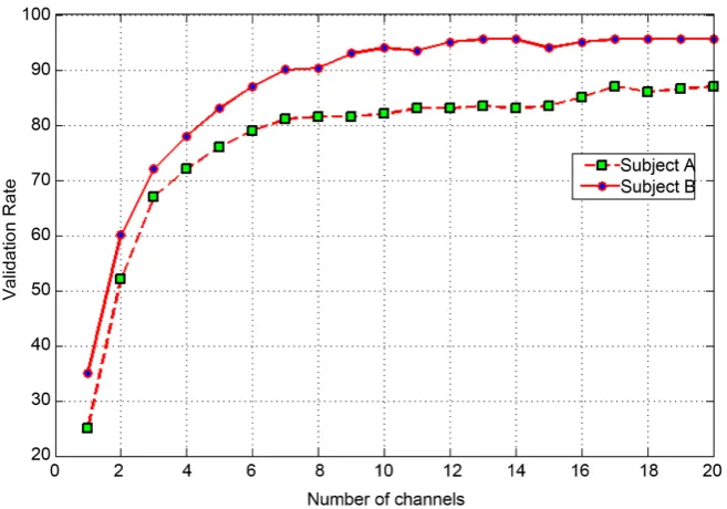
[image:5.595.210.539.474.704.2]As you see, one channel in each stage of the FBS algorithm was added to the channel set. This process continued until the optimal channel set was obtained.
Figure 3 presents validation set accuracy for first 20 channels which were ob-tained by FBS algorithm. For a proper performance, we chose channels which could create higher accuracy in validation set. According to Figure 3, 17 and 13 channels are selected for subjects A and B, respectively. Scalp position of the
selected channel set for each subject is shown in Figure 4.
3.3. Sub-Band Selection Algorithm
[image:7.595.210.540.455.698.2]P300 component doesn’t appear at the same sub-bands for different channels. On the other hand, all sub-bands in wavelet analysis don’t make enough discrimina-tion between two classes. So, using an algorithm for choosing the optimal sub- bands seems to be necessary. In this situation, not only the redundancy gotreduced in feature dimension, discrimination between two classes can increase as well. For meeting these requirements, we used Mahalanobis’s criterion which was de-fined in Equation (2).
Figure 5 shows the MD of sub-bands for selected channels in previous sec-tion. Notice that in Figure 5(a) numbers 1 to 17 of X axisreferto channels F1, F6, FC3, FCZ, C3, CZ, CP2, CPZ, CP3, P2, PZ, PO7, POZ, PO8, O1, OZ and O2, respectively. Also, in Figure 5(b) numbers 1 to 13 of X axis refer to channels FZ, FC6, C3, CZ, CPZ, P2, PO3, PO4, POZ, PO8, O1, OZ and IZ, respectively.
After computing MD of sub-bands, it is necessary to use threshold limit for optimal sub-bands selection. In order to select suitable threshold, four steps should be considered as below:
• Computing the MD of sub-bands for selected channels. Dividing area of max (MD) and min (MD) to five levels which were defined as threshold levels. • Eliminating poor sub-bands whose MD are smaller than thresholds. • Evaluating output accuracy on validation data set.
• Choosing the threshold corresponding to the best validation performance. By applying the threshold level, one can use important sub-bands with nonzero values to construct the effective features. The appropriate threshold levels were 78.36 and 45.9 for subject A and B, respectively.
Figure 5. Mahalanobis distance of different sub-bands A4, D4, D3, D2, D1 versus optimal
3.4. Classification Algorithm
We used the LDA classifier based on linear transform y = WTx to classify the feature vectors of two classes. Here, W is the discriminant vector, x is the feature vector and y is output of the LDA classifier. Fisher’s LDA defined in Equation (3), tries to obtain transformation matrix W by maximizing the ratio of between- class scatter [9]:
( )
TT bw W S W F W
W S W
= (3)
where Sb and Sw are between-class scatter matrix and within-class scatter matrix. By computing the derivative of F and setting it to zero, one can show the optimal
W is determined by below equation [10]:
(
)
1
1 2 . w
W =S−
µ µ
− (4)4. Experimental Results
4.1. Results of Dataset 1
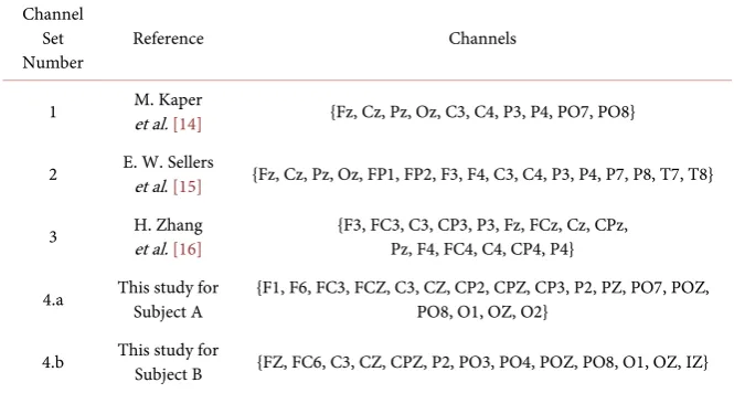
For evaluation of the proposed method in selecting optimal channel set, our channel set was compared with three other channel sets. Their list is illustrated in Table 1. Classification performances for all channel sets were computed on data set II of BCI competition [4]. This data was recorded for two different sub-jects A and B. So, the performance of each channel set is averaged between two classifiers. Results are shown in Figure 6. According to the figure, we can see that results of channel set proposed in this study are much better than others.
[image:8.595.212.541.480.702.2]To show that our proposed scheme extracts effective features, we compared the classification accuracies for all sub-bands and the optimal sub-bands as feature vectors in Table 2. According to the table, the classification accuracy of the use
of the optimal sub-bands in all trials, except in single trial, is higher than that of using all sub-bands. Besides, the feature vector dimension reduced up to 40%.
Table 3 shows a comparison between output accuracy of the two best results of the BCI competition 2005 [11], our previous work [12] and also the results obtained in this paper. As it is clear, our results are better than the second ranked competitors using SVM classifier. Although the results of this paper are some-what lower than presented results in [12], here we utilized a simple classifier and less EEG channels.
4.2. Results of Dataset 2
To investigate the robustness of the proposed method, we employed Hoffmann’s dataset [13], which was comprised of four healthy subjects and four subjects
Table 1. List of electrode positions in different channel sets.
Channel Set
Number Reference Channels
1 M. Kaper et al. [14] {Fz, Cz, Pz, Oz, C3, C4, P3, P4, PO7, PO8}
2 E. W. Sellers et al. [15] {Fz, Cz, Pz, Oz, FP1, FP2, F3, F4, C3, C4, P3, P4, P7, P8, T7, T8}
3 H. Zhang et al. [16] {F3, FC3, C3, CP3, P3, Fz, FCz, Cz, CPz, Pz, F4, FC4, C4, CP4, P4}
4.a This study for Subject A {F1, F6, FC3, FCZ, C3, CZ, CP2, CPZ, CP3, P2, PZ, PO7, POZ, PO8, O1, OZ, O2}
[image:9.595.207.539.497.578.2]4.b This study for Subject B {FZ, FC6, C3, CZ, CPZ, P2, PO3, PO4, POZ, PO8, O1, OZ, IZ}
Table 2. Evaluation the feature vector obtained by Mahalanobis’s criteria.
Feature Vector Feature Reduction Percentage of (%)
Classification Accuracy (%)
1 Trial 5 Trials 10 Trials 15 Trials
All sub-bands _ 26.5 67 85 91.5
Optimal
[image:9.595.207.541.624.733.2]sub-bands about 40 25 68 86 92
Table 3. Classification accuracy of our algorithm, the two best competitors in BCI com-petition 2005 and [12] based on the number of channels and classification algorithms.
Number of Channels
Classifier Classification Accuracy (%)
Subject A Subject B 5 Trials 15 Trials
Our scheme 17 13 LDA 68 92
First ranked [11] 64 64 SVM 73.5 96.5
Second ranked [4] 11 10 SVM 55 90.5
Our previous work
with neurological deficits. The recorded EEG data were based on visual stimuli (TV, telephone, lamp, door, window, and a radio) that evoked the P300 compo-nent. Each subject had to complete four sessions. In each session, having six runs, subjects were asked to focus on a specific image for each run, while the sequence of stimuli was randomly presented. The number of blocks inside each run was randomly chosen between 20 and 25. During every block, each image was flashed one time. The data contained 32 channels of EEG signals recorded at sampling rate of 2048. We used the data recorded in the first three sessions as the training and the last session as the test data for all eight subjects.
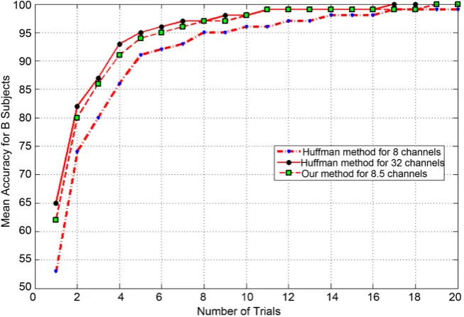
First, EEG signals were preprocessed according to Section 2. For each session, the single trial features corresponding to the first 20 blocks of flashes were ex-tracted via DWT decomposition. For each subject, we reduced the number of channels from 32 to 20 by using the sorted MD values in decreasing order. We ran the FBS algorithm (as described in Section 3.2) to choose the most effective channels from the pre-selected 20 channels. Table 4 shows the number of se-lected final channels by the proposed method for eight subjects. It is important to note that the mean number of selected channels is 8.5 per subject. In order to select the best sub-bands of decomposed coefficients (A4, D4, D3, D2, D1), the se-lected channels were used to compute the efficient threshold by using the Maha-lanobis criteria as described in Section 3.3. For each subject, we ran the sub-band selection procedure and reduced the feature vector dimension as nearly 45%. The results showed that by eliminating those sub-bands whose MD values were smaller than the threshold, the number of features was reduced without decreasing the accuracy. Moreover, in some cases, the classification accuracy was improved.
Figure 7 presents the mean accuracy for 8 subjects in our proposed scheme and Hoffman method with 8 and 32 channels.
4.3. Run Time and Computational Complexity
We compared the computation time in our approach with our previous works
[image:10.595.208.539.699.733.2][12] [17] and two best results in the BCI competition [4] [11]. The results re-vealed that the training time of our procedure was significantly lower than the first and the second ranked competitors using SVM classifier. The fact is that when training data dimension is too large, tuning of the SVM classifier is very difficult and its performance is reduced. So as to reduce the dimension of the training data in [11], the data was divided into 17 partitions, and for each parti-tion, final channels were selected among all of the 64 channels by using back-ward selection algorithm. The decision on target or non-target test data was made by voting on the outputs of 17 parallel SVM classifiers. Although this me-thod has better accuracy as compared to our scheme, it extremely increases the
Table 4. Number of selected channels for each subject.
Subjects S1 S2 S3 S4 S6 S7 S8 S9
Figure 7. The mean accuracy for 8 subjects of second dataset in our proposed method and Hoffman method for 8 and 32 channels.
computational requirements and training time. It is worth mentioning that we used fewer channels than the first ranked competitor. Additionally, we used the LDA classifier that needs less calculation as compared to the SVM. We observed that the training phase in this paper was nearly 2 and 1.5 times faster than the previous works in [12] and [17], respectively. The procedure of feature and channel selection in [17] is more complex and needs more computations than this work. The LDA outperforms the BLDA that used in [12][17] in small size data because of parameters tuning requirements of BLDA and its complexity.
5. Conclusion
ex-isting schemes.
References
[1] Wolpaw, J.R., Birbaumer, N. and Heetderks, W.J. (2000) Brain Computer Interface Technology: A Review of the First International Meeting. IEEE Trans Rehab Engi-neering, 8, 64-73. https://doi.org/10.1109/tre.2000.847807
[2] Wolpaw, J.R., Birbaumer, N., McFarland, D., Pfurtscheller, G. and Vaughan, T. (2002) Brain-Computer Interfaces (BCIs) for Communication and Control. Clinical Neurophysiology, 113, 767-791.
[3] Farwell, L.A. and Donchin, E. (1988) Talking off the Top of Your Head: Toward a Mental Prosthesis Utilizing Event-Related Brain Potentials. Electroen-Cephalogra- phy and Clinical Neurophysiology, 70, 510-523.
[4] BCI Competition III Webpage.
http://www.bbci.de/competition/iii/#data_set_iiib
[5] Schalk, G., McFarland, D., Hinterberger, T., Birbaumer, N. and Wolpaw, J.R. (2004) BCI2000: A General-Purpose Brain-Computer Interface (BCI) System. IEEE Trans-actions on Biomedical Engineering, 51, 1034-1043.
https://doi.org/10.1109/TBME.2004.827072
[6] Markazi, S.A., Stergioulas, L.K. and Ramchurn, A. (2007) Latency Corrected Wave-let Filtering of the P300 Event-Related Potential in Young and Old Adults. Pro-ceeding of the 3rd International IEEE EMBS Conferences on Neural Engineering, Hawaii, 2-5 May 2007, 582-586.
[7] Fatourechi, M., Birch, G.E. and Ward, R.K. (2007) Application of a Hybrid Wavelet Feature Selection Method in the Design of a Self-Paced Brain Interface System. Journal of Neuro Engineering and Rehabilitation, 4, 11.
https://doi.org/10.1186/1743-0003-4-11
[8] Theodoridis, S. and Koutroumbas, K. (2003) Pattern Recognition. 2nd Edition, Aca- demic Press, San Diego.
[9] Fisher, R.A. (1936) The Use of Multiple Measurements in Taxonomic Problems. Annals of Human Genics, 7, 179-188.
[10] Martinez, A. and Aka, A. (2001) PCA versus LDA. IEEE Transactions on Pattern Analysis and Machine Intelligence, 23, 228-233.https://doi.org/10.1109/34.908974 [11] Rakotomamonjy, A. and Guigue, V. (2008) BCI Competition III: Dataset II-En-
semble of SVMs for BCI P300. IEEE Transactions on Biomedical Engineering, 55, 1147-1154.https://doi.org/10.1109/TBME.2008.915728
[12] Perseh, B. and Kiamini, M. (2013) Optimizing Feature Vectors and Removal Unne-cessary Channels in BCI Speller Application. Journal of Biomedical Science and En-gineering, 6, 973-981. https://doi.org/10.4236/jbise.2013.610121
[13] Hoffmann, U., Vesin, J.M., Ebrahimi, T. and Diserens, K. (2008) An Efficient P300- Based Brain-Computer Interface for Disabled Subjects. Journal of Neuroscience Methods, 167, 115-125.
[14] Kaper, M. and Ritter, H. (2004) Generalizing to New Subjects in Brain-Computer Interfacing. Proceedings of the 26th Annual Conference in EMBS, San Francisco, 1- 4 September 2004, 4363-4366.https://doi.org/10.1109/iembs.2004.1404214
[15] Thulasidas, M. and Guan, C. (2005) Optimization of BCI Speller Based on P300 Po-tential. Proceedings of the 27th Annual Conference in Medicine and Biology, Shanghai, 1-4 September 2005, 5396-5399.
Interna-tional Conference on Natural Computation, Haikou, 24-27 August 2007, 280-284. https://doi.org/10.1109/ICNC.2007.172
Appendix
We applied validation process based on five-fold cross-validation method to ob-tain proper channels. The procedure follows items below:
• Training data with 85 × 12 × 15 × Channel Count signals (where, 85: charac-ters, 12: stimuli, 15: time repetitions, and Channel Count: number of chan-nels) averaged over all signals by 3 times repetitions. So, training data con-tained 85 × 12 × 5 × Channel Count signals.
• We divided 85 characters to five partitions and built validation set from N × 12 × 5 × Channel Count signals, where, N contains 17 characters and used residual data to form a training set.
• Feature vectors were created based on wavelet coefficients (approximate coeffi-cients level 4 and detail coefficoeffi-cients levels 1 to 4 (A4, D4, D3, D2, D1).
• The LDA classifier was trained and output precision was evaluated based on validation set. The precision is defined as: Prec Tp
TP FP FN
=
+ + , where TP, FP,
FN are the number of true positive, false positive and false negative respec-tively.
• Validation performance was assessed by averaging between five precisions.
Submit or recommend next manuscript to SCIRP and we will provide best service for you:
Accepting pre-submission inquiries through Email, Facebook, LinkedIn, Twitter, etc. A wide selection of journals (inclusive of 9 subjects, more than 200 journals)
Providing 24-hour high-quality service User-friendly online submission system Fair and swift peer-review system
Efficient typesetting and proofreading procedure
Display of the result of downloads and visits, as well as the number of cited articles Maximum dissemination of your research work