Munich Personal RePEc Archive
Maximin equilibrium
Ismail, Mehmet
Maastricht University
March 2014
Maximin equilibrium
Mehmet ISMAIL
March, 2014
Abstract
1
Introduction
In their ground-breaking book, von Neumann and Morgenstern (1944, p.555) describe the maximin strategy1 solution for two-player games as follows.
“There exists precisely one solution. It consists of all those impu-tations where each player gets individually at least that amount which he can secure for himself, while the two get together pre-cisely the maximum amount which they can secure together. Here the ‘amount which a player can get for himself’ must be under-stood to be the amount which he can get for himself, irrespective of what his opponent does, even assuming that his opponent is guided by the desire to inflict a loss rather than to achieve again.”
This immediately gives rise to the following question: ‘What happens when a player acts according to the maximin principle but knowing that other players do not necessarily act in order to decrease his payoff?’. We are going to capture this type of behavior by assuming that players are ‘rational’2
and letting it be common knowledge among players. In other words, the contribution of the current paper can roughly be considered as incorporating the maximin principle and rationality of the players in one concept calling it maximin equilibrium.
Note that it is recognized and explicitly stated by von Neumann and Morgenstern several times that their approach can be questioned by not capturing the cooperative side of non-zero-sum games. But this did not seem a big problem at that time and it is stated that the applications of the theory should be seen in order to reach a conclusion.3 After more than a
half-century of research in this area, maximin strategies are indeed considered to be too defensive in non-strictly competitive games in the literature. Since a maximin strategist plays any game as if it is a zero-sum game, this leads
1
We would like to note that the famous minimax (or maximin) theorem was proved by von Neumann (1928). Therefore, it is generally referred as von Neumann’s theory of games in the literature.
2
Throughout the text, we will specify in which context rationality is used to avoid confusion, e.g. rationality in maximin strategies, rationality in Nash equilibrium and so on. The word ‘rationality’ alone will be used when we do not attach any mathematical definition to it (until we formally define).
3
to an ignorance of her opponent’s payoffs and hence the preferences of her opponent. These arguments call for a revision of maximin strategy concept. Let us consider the following games to support our statement. In the first game4, Alfa (he) is the row player and Beta (she) is the column player.
There is a unique mixed Nash equilibrium [(34,14),(12,12)] at which Alfa re-ceives an expected payoff of 3 and Beta rere-ceives 4. On the other hand, Alfa has a unique maximin strategy (1
2, 1
2) which guarantees him to receive an
expected payoff of 3. Beta also has a unique maximin strategy (14,34) which guarantees her 4. Although the point we want to make is different, it is of importance to note the historical discussion about this type of games where Nash equilibrium payoffs are equal to the payoffs that can be guaranteed by playing maximin strategies. Harsanyi (1966) postulates that players should use their maximin strategies in those games. Aumann and Maschler (1972) state that they do not know what to recommend but maximin strategies seem preferable.
a b
a 5,1 1,5 b 1,13 5,1
In short, in the games similar as above, the arguments supporting max-imin strategies are so strong that it led some game theory giants to prefer them over the unique Nash equilibrium of the game. However, these argu-ments suddenly disappear and the weakness of maximin strategies can be easily seen if we add a strategy trick to the previous game for both players as in the following game. Let the payoffs be as given in Figure 1 with some small ǫ > 0. For every ǫ > 0 there is one completely mixed5 and one pure
Nash equilibrium (trick, trick) whose payoffs to both players are 0. The third Nash equilibrium [(34,14,0),(12,12,0)] is the same as the previous game and its payoff vector is (3,4).
However, notice that the maximin strategies of the previous game have disappeared. The new maximin strategy is trick which guarantees 0 while the other strategies guarantee−ǫ for a player. To elaborate on the reason of this, let us first see why the old Nash equilibrium survived.
4
It is strategically equivalent to the game in Aumann and Maschler (1972,p.55).
5
For example, if ǫ = 1 then mixed Nash equilibrium is [(3 20,
1 20,
4 5),(
1 8,
1 8,
3
4)] whose
a b trick
a 5,1 1,5 −ǫ,0 b 1,13 5,1 −ǫ,0
[image:5.612.233.379.127.188.2]trick 0,−ǫ 0,−ǫ 0,0
Figure 1: A game with an ǫ >0.
Suppose that players made an agreement (explicitly or implicitly) to play the Nash equilibrium [(34,14,0),(12,12,0)].6 Then, Alfa would make sure that
Beta would not unilaterally deviate to the strategy trick because Beta is rational (`a la Nash). That is, deviating gives 0 to Beta which is strictly less than what she would receive if she did not deviate. Beta would also make sure that Alfa would not make a unilateral deviation to trick for the same reason. Therefore, one observes that Nash equilibrium is immune to this sort of additions of strategies whose payoffs are strictly less than the ones of the original game.7 It may create additional Nash equilibria though. We extend
the maximin principle in such a way that it also becomes immune to these type of ‘tricks’.
To see what actually happened to the maximin strategies of the first game let us look at its profile [(1
2, 1 2,0),(
1 4,
3
4,0)] in the second game. Suppose that
players agreed (explicitly or implicitly) to play this profile. Alfa would make sure that Beta would not unilaterally deviate to the strategytrick if Beta is ‘rational’ because she receives 0 by deviating which is strictly less than what she would receive, namely 4. Beta would also make sure that Alfa would not unilaterally deviate to trick if he is ‘rational’. A player might still deviate to a or b but this is okay for both players since they both guarantee their respective payoffs in this region.8 That is, Alfa would guarantee to receive 3
given that Beta is ‘rational’ and Beta guarantees to receive 4 given that Alfa is ‘rational’.
6
Note that it is not in general known how players coordinate or agree on playing a specific Nash equilibrium. We would like to see ‘if’ they agree then what happens. As it is stated in Aumann (1990), a player does not consider an agreement as a direct signal that her opponent will follow it. But by making an agreement, she rather understands that the other player is signalling that he wants her to keep it.
7
If, for example, the payoffs totrickwere 6 instead of 0, then obviously this would not be the case.
8
In conclusion, we think that if players prefer playing their maximin strate-gies in the first game, then they would prefer playing the strategy pro-file [(12,12,0),(14,34,0)] in the second game if their ‘rationality’ is commonly known.
In Section 2, we define the rationality assumption we would like to use in this paper. In Section 3, we introduce the concept of maximin equilib-rium. Similar to maximin strategies, maximin equilibrium is a method for evaluating the uncertainty that players are facing by playing the game. We show that maximin equilibrium is invariant under strictly increasing trans-formations of the payoff functions of the players. Moreover, every finite game possesses a maximin equilibrium in pure strategies.
In Section 4, we consider the games in von Neumann-Morgenstern mixed extension and discuss the relationship of maximin equilibrium with the other solution concepts. We show that maximin equilibrium is a coarsening of Nash equilibrium. Moreover, we demonstrate that maximin equilibrium coincides with Nash equilibrium in two-player zero-sum games. We also propose a refinement of maximin equilibrium called strong maximin equilibrium. Ac-cordingly, we show that for every Nash equilibrium that is not a strong maximin equilibrium there exists a strong maximin equilibrium that Pareto dominates it. In addition, no strong maximin equilibrium is ever Pareto dominated by a Nash equilibrium. Furthermore, we show by examples that maximin equilibrium is neither a coarsening nor a special case of correlated equilibrium or rationalizable strategy profiles.
In Section 5, we discuss the maximin equilibrium in extensive form games and in n-player games. All the results provided in Section 3 and in Section 4 hold in n-player games except the one which requires a two-player zero-sum setting. Finally, we discuss maximin equilibrium predictions in several games including the traveler’s dilemma.
2
The framework
In this paper, we use a framework for the analysis of interactive decision making environments as described by von Neumann and Morgenstern (1944, p.11).
footnote 2 on p. 10, by a mere recourse to the devices of the the-ory of probability. Every participant can determine the variables which describe his own actions but not those of the others. Nev-ertheless those ‘alien’ variables cannot, from his point of view, be described by statistical assumptions. This is because the others are guided, just as he himself, by rational principles –whatever that may mean– and no modus procedendi can be correct which does not attempt to understand those principles and the interac-tions of the conflicting interests of all participants.
For simplicity, we assume that there are two players whose finite set of pure actions are X1 andX2 respectively. Moreover, players’ preferences over
the outcomes are assumed to be a weak order (i.e. transitive and complete) so that we can represent those preferences by the (ordinal) utility functions
u1, u2 : X1 ×X2 → R which depends on both player’s actions. As usual,
the notation x in X = X1 ×X2 represents a strategy profile. In short, a
two-player non-cooperative game can be denoted by ({1,2}, X1, X2, u1, u2).
Starting from simple strategic decision making situations, we firstly introduce a deterministic theory of games in this section and in the following one.9
For the analysis of a game we need a notion of ‘rationality’ of the players. Moreover, we assume that players maximize utility with respect to the worst case given that the ‘rationality’ of the players is common knowledge. We assume that everything about the game including the previous sentence is common knowledge.10
In one-player decision making situations the notion of rationality is usu-ally referred as maximizing one’s own utility with respect to her preferences. In multi-player games, however, it is not unambiguous what does it mean to maximize one’s own utility because it simply depends on the other’s ac-tions. Von Neumann proposed proposed an approach to do this: Each player should maximize a minimum utility regardless of the strategy of the other player. Although, in two-player zero-sum games this works quite well, it is considered to be too pessimistic in non-zero-sum games since the preferences
9
Note that all the definitions we present can be extended in a straight-forward way to the games in von Neumann-Morgenstern mixed extension and to n-player games. See Section 4 and in the Section 5 for more discussion. Note also that interpreting utilities as cardinal which is usual in game theory does not cause any problems.
10
of the players are not necessarily opposing. Due to the fact that rationality of the maximin strategist dictates her to play any game as if it is a zero-sum game, this leads her to ignore the opponent’s payoffs and hence the prefer-ences of the opponent. Therefore, one might call maximin strategist being an individually rational player who does not, in general, take the advantage of all the information given to her.
2.1
Definition of rationality
To avoid possible misunderstandings from our rationality definition, one may consider the following scenario in mind which is intended only to facilitate the definition.
Suppose that Alfa and Beta are sitting at a bargaining table and can make non-binding agreements. However, they will submit their strategies in separate rooms simultaneously. By making an agreement on a strategy profile and going back to their rooms, each player faces a decision problem of either keeping the agreement or betraying it by a deviation. Accordingly, we discuss what would players do if they are rational in the sense of maximin strategy, Nash equilibrium and of the notion we define as maximin equilibrium.
Firstly, if the players are rational `a la von Neumann, then a player is expected to betray an agreement by deviating to any strategy (including the ones which he gets a strictly less payoff than the agreement payoff). The reason is obvious: Maximin rule imposes no condition on the other player’s strategies. Secondly, if we assume that players are rational `a la Nash, then a player is expected to betray the agreement unless he is already best replying. Note that these are two extreme cases that might occur: In the former, there is no condition on the strategy of the other player while there is unique condition in the latter one. We define a rationality concept which is stronger than of maximin strategist but weaker than of Nash strategist. According to our definition, a rational player will be the one who would not betray the agreement by making a non-profitable deviation. 11
Let us fix some terminology. As usual, a strategy x′
i ∈ Xi is said to
be a profitable deviation for player i with respect to the profile (xi, xj) if
ui(x′i, xj)> ui(xi, xj). We call it non-profitable if it is not profitable.
11
Definition 1. A player is called rational at (the agreement) x if she does not make a non-profitable deviation from it.
In other words, when Alfa and Beta leave the bargaining table, Alfa would make sure that Beta would not betray the agreement by deviating non-profitably if Beta is rational and vice versa.
The reader might ask whether we need to assume that pre-play communi-cation is allowed. The answer is that we do not need it; an agreement can be explicit or implicit. The assumptions of rationality and players being max-imin decision makers are, basically, the ‘rules’ that players take into account in order to reach an agreement. Since those rules are fixed and common knowledge, players can make the same reasoning in the lack of communica-tion as they do in the presence of a communicacommunica-tion.
At first sight, it might seem subtle that a player makes a reasoning about a strategy profile which actually includes her own strategy in the above inter-pretation. However, careful examination reveals that it is not a problem since she is reasoning about a possibility that she makes an agreement. Initially, every strategy profile is a potential agreement.
3
Maximin equilibrium
As it is formulated and explained by von Neumann (1928), playing a game is basically facing an uncertainty which can not be resolved by statistical assumptions. This is actually the crucial difference between games and deci-sion problems. Our aim is to extend von Neumann’s approach on resolving this uncertainty.
Suppose that Alfa and Beta make a non-binding agreement (x1, x2).
Alfa faces an uncertainty by keeping the agreement since he does not know whether Beta will keep it. Von Neumann’s method to evaluate this uncer-tainty is to calculate the minimum payoff of Alfa with respect to all conceiv-able deviations by Beta.12 That is, Alfa’s evaluation v
x1x2 (or the utility)
of keeping the agreement (x1, x2) is vx1x2 = minx′2∈X2u1(x1, x
′
2). Note that
for all x′
2, the evaluation of Alfa for the profile (x1, x′2) is the same, i.e.
vx1x2 = vx1x′2 for all x
′
2 ∈ X2. Therefore, it is possible to attach a unique
evaluation vx′1 for every strategy x′1 ∈ X1 of Alfa. Next step is to make a 12
comparison between those evaluations of the strategies. For that, von Neu-mann takes the maximum of all such evaluationsvx′1 with respect tox′1 which
yields a unique evaluation for the whole game, i.e. the value of the game is
v = maxx′
1∈X1vx′1. In other words, the unique utility that Alfa can guarantee
by facing the uncertainty of playing this game is v. Accordingly, it is rec-ommended that Alfa should choose the strategyx∗
1 ∈arg maxx′1∈X1vx′1 which
guarantees the value v.
We would like to extend von Neumann’s method in such a way that Alfa takes into account the rationality of Beta when making the evaluations and vice versa. Let us construct the approach we take step by step and state its implications.
Firstly, one needs to define the rationality. We have chosen a notion of rationality which allows Beta to keep her agreement or to deviate to a strategy for which she has strict incentives to do so. By this assumption, Alfa can rule out non-profitable deviations of Beta from the agreement (x1, x2) which helps
decreasing the level of uncertainty he is facing. Now, Alfa’s evaluation vx1x2
of the uncertainty for keeping the agreement can be defined as the minimum utility he would get under any rational behavior of Beta. That is,
vx1x2 = min{ min
x′
2∈B2(x1,x2)
u1(x1, x′2), u1(x1, x2)}},
where B2(x1, x2) denotes the set of Beta’s (strict) better replies with respect
to (x1, x2). As a consequence, it is not in general true for a strategy x′2 6=x2
that we have the equality vx1x2 = vx1x′2. Because, the better response set
of Beta with respect to (x1, x2) is not necessarily the same as the better
response set of her with respect to (x1, x′2). Therefore, we can not assign a
unique value to every strategy of Alfa anymore. Instead, the evaluation of the uncertainty can be encoded in the strategy profile. As a result, we can no longer refer a strategy in the same sprit of a maximin strategy since a strategy in this setting only makes sense as a part of a strategy profile.13 But note
that there are two evaluations that are attached to the profile (x1, x2), one
from Alfa and one from Beta since she also is doing the similar calculations as him. Accordingly, we define a value function which maps each strategy profile to a vector whose components represent the value of the profile to each player.
13
The last step is to make comparisons between those evaluations. Our aim is basically to maximize the value function but since it is vector valued there is no obvious way to do this. At first sight, it might seem that we have not done a big improvement so far since we have started with a maximization of payoff vectors of the players but we are still left with a similar problem. However, we can now use the maximization (optimization) methods we know in the literature just as techniques. Two well-known maximization techniques are Pareto optimality and Nash equilibrium.
One may ask why we do not directly apply those maximization methods to the set of payoff vectors of the game. The reason is that applying a maximization method to a game does not necessarily mean evaluating and comparing the uncertainty that a player faces by playing according to what it recommends.
For example, let the strategy profile z be Pareto optimal in the whole domain of a game. Even though the payoff that Alfa receives from the profile
z is high, playing her part of the Pareto optimal profile need not be a good (utility maximizing) decision ex ante. Because, the uncertainty he faces by playing his part is not evaluated. For example, it could be the case that Beta has a chance to deviate from z which causes a substantial decrease in his payoff. Therefore, it would be better for Alfa if he considers his possible payoffs after such deviations and compare it with the other possible options. To give another example, let now w be a Nash equilibrium. Again, the fact that w is a Nash equilibrium does not make playing his part of w a good decision for Alfa. Alfa needs to evaluate the uncertainty he is facing by playing his part and compare it with the other options. Actually, it is better to call it a certainty rather than an uncertainty because of the fact that neither Beta nor Alfa has a profitable deviation from it. However, it is still an unevaluated and uncompared certainty in the game.
Loosely speaking, choosing the Nash equilibrium in the presence of many other strategy profiles is like choosing the sure gamble in the presence of many other uncertain gambles. Even if the outcomes of the uncertain gamble is very high in every state of the world and the outcome of the sure gamble is very low.
Nash’s method only compares the outcomes that might occur as a conse-quence of a player choosing one strategy with the outcomes that might occur as a consequence of an opponent choosing another strategy.14 Therefore, a
14
Nash equilibrium completely ignores the outcomes that might occur under any other strategy choices of the players no matter how high their utilities are. If, by any chance, there is only one Nash equilibrium, then this ignorance might lead to a disastrous outcome for both players. One can see this clearly in the traveler’s dilemma game which was introduced by Basu (1994).15 If
players play the unique Nash equilibrium, then they ignore a large part of the game which is actually profitable for both of them. At the end of the day, what a utility maximizing player cares is the payoff she receives not the nice property of being sure that her opponent would not deviate had they agreed to play a profile.
Another question one might ask is why we use both Pareto optimality and Nash equilibrium methods for maximization of the value function. The answer is that we simply want to minimize potential disadvantages of using only one of the two. It is well-known that Pareto optimality sometimes yields quite unfair outcomes and that a Nash equilibrium outcome can be quite unsatisfactory. Let us now define the value function formally.
Definition 2. Let Γ = (X1, X2, u1, u2) be a two-player game. A function
v :X →R×R is called the value function of Γ if for every i6=j and for all
x= (xi, xj)∈X, i’th component of v = (vi, vj) satisfies
vi(x) = min{ min x′
j∈Bj(x)
ui(xi, x
′
j), ui(x)}},
where the better response correspondence of player j with respect to x is defined as
Bj(x) = {x′j ∈Xj|uj(xi, x′j)> uj(x)}.
Remark 3. Note that for all xand all i, we have ui(x)≥vi(x). Because, one
cannot increase a payoff but can only (weakly) decrease it, by definition of the value function.
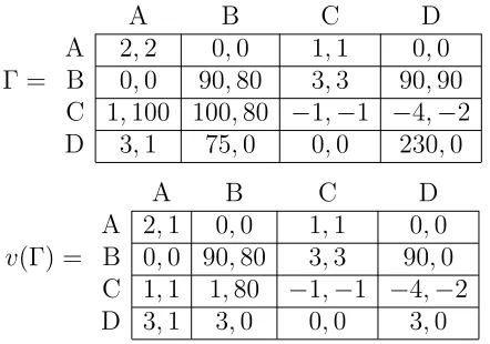
As it is discussed above, the value of a strategy profile to a player repre-sents the minimum payoff that a player could receive under rational behavior of her opponent. To illustrate what a value function of a game looks like, let us consider the game in Figure 2 which is played by Alfa and Beta.
15
Γ =
A B C D
A 2,2 0,0 1,1 0,0 B 0,0 90,80 3,3 90,90 C 1,100 100,80 −1,−1 −4,−2 D 3,1 75,0 0,0 230,0
v(Γ) =
A B C D
[image:13.612.196.417.126.281.2]A 2,1 0,0 1,1 0,0 B 0,0 90,80 3,3 90,0 C 1,1 1,80 −1,−1 −4,−2 D 3,1 3,0 0,0 3,0
Figure 2: A game Γ and its value function v(Γ).
Observe that Γ has a unique Nash equilibrium (D,A) whose payoff vector is (3,1). Suppose that pre-game communication is allowed and that Beta is trying to convince Alfa at the bargaining table to make an agreement on playing, for example, the profile (C,B) which Pareto dominates the Nash equilibrium. Alfa would fear that Beta may not keep his agreement and may unilaterally deviate to A leaving her a payoff of 1. Accordingly, the value of the profile (C,B) to Alfa is 1 as shown in the bottom table in Figure 2. Since agreements are not binding, Alfa would not accept this agreement. Now, suppose Alfa offers to make an agreement on (B,B). Beta would not fear a unilateral profitable deviation C of Alfa since his payoff does not decrease in that case. Alfa’s payoff does not decrease too in case of a unilateral profitable deviation of Beta to D. In other words, the value of the profile (B,B) is (90,80) which is equal to its payoff vector in Γ.
Now, we are ready to define the maximin equilibrium.
Definition 4. A strategy profile x = (xi, xj) where i 6= j in a two player
game Γ is called maximin equilibrium if it satisfies at least one of the following conditions for the value function v = (vi, vj):
1. For every playeri and allx′
∈X, vi(x′)> vi(x) impliesvj(x′)< vj(x).
2. For every i, xi ∈arg maxx′
i∈Xivi(x
′
i, xj).
Remark 5. We can interpret the value functionv of a game Γ as a game in its own right, that is, Γv = (X1, X2, v1, v2) where v(Γ) = (v1, v2). Then, the set
of maximin equilibria in Γ is the union of the set of Pareto optimal strategy profiles and the set of Nash equilibria of the game Γv.
Going back to our example, observe that the profile (B,B) is the Pareto dominant profile of the value function of the game Γ shown in Figure 2, so it is a maximin equilibrium. In addition, observe that the Nash equilibrium is also a maximin equilibrium. Moreover, the maximin equilibrium (B,B) has another property which deserves attention. Suppose that players agree on playing it. Alfa has a chance to make a unilateral profitable deviation to C but he can not rule out a potential profitable deviation of Beta to the strategy D. If this happens, Alfa would receive −4 which is less than what he would receive if he did not deviate. But Beta is also in the exactly same situation. As a result, nobody would actually deviate from the agreement (B,B).
An ordinal utility function is unique up to strictly increasing transforma-tions. Therefore, it is crucial for a solution concept (which is defined with respect to ordinal utilities) to be invariant under those operations. The fol-lowing proposition shows that maximin equilibrium possesses this property.
Proposition 6. Maximin equilibrium is invariant under strictly increasing
transformations of the payoff function of the players.
Proof. Let Γ = (Xi, Xj, ui, uj) and ˆΓ = (Xi, Xj,uˆi,uˆj) be two games such
that ˆui and ˆuj are strictly increasing transformations of ui and uj
respec-tively. Firstly, we show that the components ˆvi and ˆvj of the value function
ˆ
v are strictly increasing transformations of the components vi and vj of v,
respectively. Notice that,
Bj(x) ={x
′
j ∈Xj|uj(xi, x
′
j)> uj(x)}
= ˆBj(x) ={x
′
j ∈Xj|uˆj(xi, x
′
j)>uˆj(x)}.
It implies that arg minx′j∈Bj(x)ui(xi, x
′
j) = arg minx′j∈Bˆj(x)uˆi(xi, x
′
j). It in turn
implies that vi(x) = min{ui(xi,x¯j), ui(x)}and ˆvi(x) = min{uˆi(xi,x¯j),uˆi(x)}
for some ¯xj ∈arg minx′
j∈Bj(x)ui(xi, x
′
j).
Since ˆuiis a strictly increasing transformation ofui, we have eithervi(x) =
ui(xi,x¯j) if and only if ˆvi(x) = ˆui(xi,x¯j) or vi(x) = ui(x) if and only if
ˆ
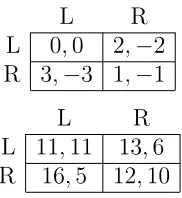
L R L 0,0 2,−2 R 3,−3 1,−1
L R
[image:15.612.263.354.125.224.2]L 11,11 13,6 R 16,5 12,10
Figure 3: Two ordinally equivalent games.
It follows that showing vi(x) ≥ vi(x′) if and only if ˆvi(x) ≥ ˆvi(x′) is
equivalent to showing ui(x)≥ui(x′) if and only if ˆui(x)≥uˆi(x′) for all x, x′
in X which is correct by our supposition.
Secondly, a profile y is a Pareto optimal profile with respect to v if and only if it is Pareto optimal with respect to ˆv because each vi is a strictly
increasing transformation of ˆvi. By the same argument, a profile y is a pure
Nash equilibrium in the game Γv if and only if it is a pure Nash equilibrium
in Γˆv. As a result, the set of maximin equilibria of Γ and ˆΓ are the same.
The following proposition shows the existence of strong maximin equi-librium hence the existence of maximin equiequi-librium with respect to pure strategies. It is especially of importance in games where players can not or are not able to use a randomization device. It might be also the case that a commitment of a player to a randomization device is implausible. In those games, we can make sure that there exists at least one maximin equilibrium.
Theorem 7. Every finite game has a strong maximin equilibrium.
Proof. Since the Pareto dominance relation is transitive a Pareto optimal strategy profile with respect to the value function of a finite game always exists.
100 99 · · · 3 2 100 100,100 97,101 · · · 1,5 0,4
[image:16.612.210.409.127.221.2]99 101,97 99,99 · · · 1,5 0,4 ... ... ... . .. ... ... 3 5,1 5,1 · · · 3,3 0,4 2 4,0 4,0 · · · 4,0 2,2
Figure 4: Traveler’s dilemma
however, after the coin toss player 1 still needs to make a decision whether playing according to the outcome of the toss or not. Actually, playing the strategy R guarantees more than playing L after the toss. Confirming the intuitions about the game in Figure 3, the pure maximin equilibrium of this game is (R,R). However, note that if the utility functions of a zero-sum game are ordinal, then the usual intuition of zero-sum games may not hold. For example, the game on the bottom in Figure 3, is ordinally equivalent to the zero-sum game on the top.
Let us now look at the traveler’s dilemma game in Figure 4. The payoff function of a player i if she plays xi and her opponent plays xj is defined
as ui(xi, xj) = min(xi, xj) + 2sgn(xj −xi) for all xi, xj in {2,3, ...,100}. In
this game, the unique strict Nash equilibrium is (2,2) which is also the only rationalizable strategy profile. To find the maximin equilibria we first need to compute the value of the traveler’s dilemma game. With appropriate calculations, one can observe that profiles (100,100) and (2,2) are maximin equilibria. The profile (100,100) is the strong maximin equilibrium whose value is (97,97).16
It is shown by many experiments that the players do not on average choose the Nash equilibrium strategy but choose 100 or something close to 100. Note that changing the reward/punishment level (which is 2 in the example) effects the behavior observed in experiments. Goeree and Holt (2001) found that when reward is high 80% of the subjects choose the Nash equilibrium strategy but when reward is small about 80% of the subjects choose the highest. This finding is a confirmation of Capra et al. (1999), that is, when reward was high the play converged towards the Nash equilibrium over time but when
16
reward level was small the play converged towards the other extreme. On the other hand, Rubinstein (2007) found (in a web-based experiment without payments) that 55% of 2985 subjects choose the highest amount and only 13% choose the Nash equilibrium where the reward was small.
These results are actually not unexpected. The irony is that if both players choose almost17 any ‘irrational’ strategy but their Nash equilibrium strategy then they both get strictly more payoff than they would get by playing the Nash equilibrium. Actually, the Nash equilibrium is the only profile which has this property. Therefore, it is difficult to imagine that a player whose aim is to maximize her own payoff would ever play or expect her opponent to play the strategy 2 in this game unless she is a ‘victim’ of game theory.
4
Maximin equilibrium in mixed strategies
4.1
Definition
The mixed extension of a two-player non-cooperative game is denoted by (∆X1,∆X2, u1, u2) where ∆Xi is the set of all simple probability
distribu-tions (lotteries) over the set Xi. It is assumed that the preferences of the
players over the lotteries satisfy weak order, continuity and the independence axioms.18 As a result, those preferences can be represented by von
Neumann-Morgenstern (expected) utility functions u1, u2 : ∆X1 × ∆X2 → R. Let
p∈∆X denote a strategy profile where ∆X = ∆X1×∆X2.
We do not need another definition for maximin equilibrium with respect to mixed strategies; one can just interpret the strategies in the Definition 4 as being mixed. But we need to modify the value function as follows to have it well defined. The value function of player i is defined as vi(p) =
min{infp′j∈Bj(p)ui(pi, p
′
j), ui(p)}} for all p∈∆X.19
Harsanyi and Selten (1988, p.70) argue that invariance with respect to positive linear transformations of the payoffs is a fundamental requirement for a solution concept. The reason is obvious: The von Neumann-Morgenstern utility function of a player is unique up to positive linear transformations.
17
If one modifies the payoffs of the game such that ui(xi,3) = 2.1 for all i and all
xi∈ {4,5, ...,100}. Then, one can remove ‘almost’ from the sentence.
18
For more information see, for example, Fishburn (1970).
19
The following remark states that maximin equilibrium has this property. We do not provide a proof since it follows essentially the same steps as the proof of Proposition 6.
Remark 8. The maximin equilibria of a game in mixed extension is unique up to positive linear transformations of the payoffs.
The following lemma illustrates a useful property of the value function of a player.
Lemma 9. The value function of a player is upper semi-continuous.
Proof. In several steps, we show that the value function vi of player i in a
game Γ = (∆X1,∆X2, u1, u2) is upper semi-continuous.
Firstly, we show that the better reply correspondenceBj : ∆Xi×∆Xj ։
∆Xj is lower hemi-continuous. For this, it is enough to show the graph of
Bj defined as follows is open.
Gr(Bj) ={(pj, q)∈∆Xj×∆X|pj ∈Bj(q)}.
Gr(Bj) is open in ∆Xj ×∆X if and only if its complement is closed.
Let [(pj, qi, qj)k]∞k=1 be a sequence in [Gr(Bj)]c = (∆Xj × ∆X) \Gr(Bj)
converging to (pj, qi, qj) wherepjk ∈/ Bj(qk) for all k. It follows that we have
uj(pkj, qki)≤ uj(qk) for all k. Continuity of uj implies that uj(pj, qi)≤uj(q)
which meanspj ∈/Bj(q). Hence [Gr(Bj)]c is closed which impliesBj is lower
hemi-continuous.
Next, we define ˆui : ∆Xj ×∆Xi×∆Xj →R by ˆui(pj, qi, qj) :=ui(pj, qi)
for all (pj, qi, qj) ∈ ∆Xj ×∆Xi ×∆Xj. Since ui is continuous, ˆui is also
continuous. In addition, we define ¯ui : Gr(Bj) → R as the restriction of ˆui
to Gr(Bj), i.e. ¯ui = ˆui|Gr(Bj). The continuity of ˆui implies the continuity of
its restriction ¯ui which in turn implies ¯ui is upper semi-continuous.
By the theorem of Berge (1963, p.115)20 lower hemi-continuity of B
j
and lower semi-continuity of −u¯i : Gr(Bj) → R implies that the function −v¯i : ∆Xi×∆Xj → R defined by −¯vi(q) := suppj∈Bj(q)−u¯i(pj, q) is lower semi-continuous.21 It implies that the function ¯v
i(q) = infpj∈Bj(q)u¯i(pj, q) is upper semi-continuous.
20
We follow a version of the theorem as presented in Aliprantis and Border (1994, p.569).
21
The value function of player i defined by vi(q) := min{¯vi(q), ui(q)} is
upper semi-continuous because the minimum of two upper semi-continuous functions is also upper semi-continuous.
The following theorem shows that strong maximin equilibrium and hence maximin equilibrium exists in mixed strategies.
Theorem 10. Strong maximin equilibrium exists in mixed strategies.
Proof. Let us define vmax
i := arg maxq∈∆Xvi(q) which is a non-empty
com-pact set because ∆X is compact andvi is upper semi-continuous by Lemma
9. Since vmax
i is compact and vj is also upper semi-continuous the set
vmax
ij := arg maxq∈vmax
i vj(q) is non-empty and compact. Clearly, the pro-files in vmax
ij are Pareto optimal with respect to the value function which
means vmax
ij is a non-empty compact subset of the set of strong maximin
equilibria in the game Γ. Similarly, one may show that the set vmax
ji is also a
non-empty compact subset of the set of strong maximin equilibria.
Now, let us assume that players can use mixed strategies in the game Γ in Figure 2. An interesting phenomenon occurs if we change, ceteris paribus, the payoff ofu1(C, D) from−3 to−4. Let us call the new game ˆΓ. It has the same
pure Nash equilibrium (D,A) as Γ plus two mixed one. The Pareto dominant Nash equilibrium is [(0,4146,465,0),(0,4752,0,525)] whose expected payoff vector is (90,80).22 The question arises: What is the ceteris paribus effect of increasing
the payoff of u1(C, D) from−4 to−3 on the nature of this strategic decision
making situation that it decreases the payoffs of the players dramatically in Nash equilibria? Note that by passing from ˆΓ to Γ we just slightly increase Alfa’s relative preference of the worst outcome (C,D) with respect to the other outcomes. On the other hand, there is a maximin equilibrium [B,(0,2831,0,313)] in Γ whose value is approximately 80.9 for both players. Moreover, it remains to be a maximin equilibrium with the same value in ˆΓ.23
22
The other Nash equilibrium is approximately [(0,0.01,0.001,0.98),(0.20,0.88,0,0.09)] whose expected payoff vector is approximately (88.11,1.14). The Nash equilibria are calculated via Gambit.
23
4.2
The relation of maximin equilibrium with the other
concepts
Perhaps, Nash equilibrium is one of the most well-known solution concept in game theory. Nash’s path-breaking theorem says that every finite game in mixed extension possesses at least one Nash equilibrium.
Remark 11. The value of a Nash equilibrium is the same as its payoff vector because no player can unilaterally deviate from a Nash equilibrium.
The following proposition shows that maximin equilibrium is a general-ization of Nash equilibrium.
Proposition 12. Every Nash equilibrium is a maximin equilibrium.
Proof. Let (pi, pj) be a Nash equilibrium. By Remark 11, the value of it is the
same as its payoff vector. Accordingly, we have pi ∈arg maxp′
i∈∆Xivi(p
′
i, pj)
for all player i because the values of the other profiles can not increase by Remark 3. Hence, the profile (pi, pj) is also a maximin equilibrium.
The following two propositions show the Pareto dominance relation be-tween Nash equilibrium and strong maximin equilibrium.
Proposition 13. For every Nash equilibrium that is not a strong maximin
equilibrium there exists a strong maximin equilibrium that Pareto dominates it.
Proof. If a Nash equilibrium q in a game Γ is not a strong maximin equi-librium, then there exists a strong maximin equilibrium p whose value v(p) Pareto dominates v(q). It implies that p Pareto dominates q in the game Γ since the payoff vector of the Nash equilibrium q is the same as its value by Remark 11.
Proposition 14. No strong maximin equilibrium is ever Pareto dominated
by a Nash equilibrium.
The two propositions above are closely linked but one does not follow from the other. Because, Proposition 13 does not exclude the existence of a Nash equilibrium that is both Pareto dominated by a strong maximin equilibrium and Pareto dominates another strong maximin equilibrium. Proposition 14 shows that this is not the case.
The next proposition illustrates that in zero-sum games a possibly mixed strategy is a Nash equilibrium if and only if it is a maximin equilibrium.
Proposition 15. In a two-player zero-sum game, a profile is a maximin
equilibrium if and only if it is a Nash equilibrium.
Proof. ‘⇒’ By contraposition, suppose that the strategy profile (p1, p2) is
not a Nash equilibrium, we show that it can not be a maximin equilibrium. Firstly, we show that the value of (p1, p2) is always Pareto dominated. Let
(¯p1,p¯2) be a Nash equilibrium whose payoff vector is (w,−w). Suppose,
without loss of generality, that u1(p1, p2) < w and u2(p1, p2) > −w. Next,
player 1 can profitably deviate to her maximin strategy ¯p1 from which she will
receive at least w. It implies that the value of the profile (p1, p2) for player 2
is at most −w. By Remark 3, we havev1(p1, p2)≤u1(p1, p2). It implies that
the value of the profile (p1, p2) is Pareto dominated by the value of the Nash
equilibrium (¯p1,p¯2). Secondly, the value of the profile (¯p1, p2) for player 1 is
strictly more than the value of (p1, p2), that isv1(¯p1, p2)> v1(p1, p2) because
v1(¯p1, p2) = w. Since the profile (p1, p2) also violates the second condition in
the definition of maximin equilibrium, it can not be a maximin equilibrium. ‘⇐’ By Proposition 15, every Nash equilibrium is a maximin equilibrium.
Rationalizable strategy profiles and correlated equilibrium are two differ-ent generalizations of the Nash equilibrium.24 One might wonder the
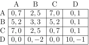
rela-tionship of maximin equilibrium with those concepts. First of all, neither rationalizable strategy profiles nor correlated equilibrium is a coarsening of maximin equilibrium. The reason is that, a strictly dominated strategy can be a part of a maximin equilibrium. For example, the profiles (A, C) and (B, D) are pure maximin equilibria in the game in Figure 5. But notice that the strategy A of player 1 is strictly dominated. Moreover, maximin equilibrium is not a generalization of ratonalizable strategy profiles. Con-sider the game in Figure 6 which is taken from Bernheim (1984) and observe
24
C D A 6,8 0,0 B 8,6 1,7
Figure 5: Example of a maximin equilibrium which include a strictly domi-nated strategy.
A B C D
A 0,7 2,5 7,0 0,1 B 5,2 3,3 5,2 0,1 C 7,0 2,5 0,7 0,1 D 0,0 0,−2 0,0 10,−1
Figure 6: A rationalizable strategy profile which is not a maximin equilib-rium.
that (A, A) is a rationalizable strategy profile, however, it is not a maximin equilibrium. Correlated equilibrium is also not a special case of maximin equilibrium either because a correlated distribution can not be a maximin equilibrium.
One might wonder whether there is a relationship between the maximin (minimax) decision rule25 in decision theory and the maximin equilibrium.
Imagine a one-person game in which the decision maker is to make a choice between several gambles. In that case, maximin equilibrium boils down to expected utility maximization just like maximin strategies and Nash equi-librium. In other words, the decision maker has to choose the gamble with the highest expected utility. However, according to maximin decision rule, a player has to choose the gamble which maximizes the utility with respect to the worst state of the world (whose outcome is the minimum) even though the probability assigned to it is very small.
25
Accept Reject Accept 16,16 16,16
Reject 16,16 Γ′
Γ′
=
Stay silent Deny Confess Stay silent 100,100 110,105 0,15
[image:23.612.177.433.126.236.2]Deny 105,110 95,95 5,380 Confess 15,0 380,5 10,10
Figure 7: Modified prisoner’s dilemma Γ in extensive form.
5
Maximin equilibrium in extensive form and
in n-player games
5.1
Extensive form games
It is possible to apply the logic of maximin equilibrium in extensive form games but we have to be careful with the definition of a profitable deviation. Because, if a player plays a strategy out of an agreement, then the other player could be informed about this before waiting the end of the game. Accordingly, the non-deviator has a chance to deviate too. Thus, defining profitable deviations via its normal form would cause a loss of information. Without getting into the heavy notation of extensive form games, we would like to present a simple example to illustrate the maximin equilibria solutions. In this example, we modify the famous prisoner’s dilemma game as fol-lows. Each player has three options to choose, namely ‘stay silent’ (S), ‘deny’ (D) or ‘confess’ (C). In addition, we add another feature: Before playing the actual game, each player is offered to choose ‘Accept’ (A) or ‘Reject’ (R). If one of them accepts, then they will both stay 12 years in prison and the actual game will not be played. If both of them reject, then they will play the game. All this information is common knowledge to both players. This situation can be represented by a two-player symmetric game in extensive form which is shown in Figure 7.26
Firstly, observe that the game Γ′
has a unique Nash equilibrium (C,C)
26
We assume that players’ utility is decreasing in the number of years that will be spent in prison. Notice that if the strategy ‘stay silent’ is removed from the game Γ′ for
with a payoff vector of (10,10). Accordingly, the unique subgame perfect Nash equilibrium of Γ is (AC,AC) whose payoff vector is (16,16). For sim-plicity, let us consider the game in pure strategies. There are four maximin equilibria (C,C), (D,S), (S,D) and (S,S) in the game Γ′
. The maximin equi-libria of Γ are (AC,AC), (RD,RS), (RS,RD) and (RS,RS) whose values are (16,16),(5,110),(110,5) and (100,100) respectively.
Suppose that both prisoners are in the same cell and they can freely discuss what to choose before their decision is asked about accepting or re-jecting the offer. However, they will make their choices in separate cells, that is, non-binding pre-game communication is allowed. We would expect that players would try to convince each other to play a strategy profile that Pareto dominates (AC, AC) because each of them can simply guarantee receiving 16 no matter what.
A potential agreement in this game seems to be the maximin equilibrium (RS,RS). It simply guarantees a payoff of 100 for a player given that his opponent is rational. First of all, a rational player would not unilaterally deviate from this agreement by playing ‘Accept’ in the beginning because it is not a profitable deviation. Moreover, if a player wants to play (A), it does not make sense for him to make an agreement since any choice of the opponent does not change the outcome. In the second stage game Γ′
, a rational player would not unilaterally deviate to C from the agreement (S,S) since it is a non-profitable deviation. He may rationally deviate to D but this is not a problem (even preferable) for the non-deviator as he gets strictly more than the value of 100. Actually, the fact that they have already rejected receiving 16 is a signal for not playing according to the Nash equilibrium.
5.2
N-player games
In this subsection, we discuss the extensions of the definitions and of the results we have presented so far to n-player games.
Regarding the definition of the value function, one only needs to replace the way vi is written in Definition 4 to,
vi(p) = min{ inf p′
−i∈B−i(p)
ui(pi, p
′
−i), ui(p)}},
where B−i(p) is the set of (n−1)-tuple strategy profiles which can occur
that is
B−i(p) = {pˆ−i ∈∆X−i|pˆk∈Bk(p) for at least one k ∈ {−i}}.27
The definition of the maximin equilibrium does not change. In other words, the set of maximin equilibria in a game Γ is the union of the set of Pareto optimal strategy profiles and the set of Nash equilibria of the game defined by the value function of Γ. Moreover, every result in Section 3 and in Section 4 except the Proposition 15 (which requires a two-player zero-sum setting) is valid in n-player games. That is, maximin equilibrium exists in pure strategies, it is invariant under strictly increasing transformations of the payoff functions of the players and it is a generalization of the Nash equilibrium in mixed strategies. Moreover, for every Nash equilibrium that is not a strong maximin equilibrium there exists a strong maximin equilibrium that Pareto dominates it. Besides, no strong maximin equilibrium is ever Pareto dominated by a Nash equilibrium. The proofs are essentially the same as the ones given in Section 3 and in Section 4.
6
Conclusion
In this paper, we have introduced a new solution concept called maximin equilibrium which extends von Neumann’s maximin strategy idea to n-player games by incorporating common knowledge of rationality of the players. The rationality assumption we use is stronger than the one of maximin strate-gist and weaker than the one of Nash stratestrate-gist. Maximin equilibrium is a method for evaluating the uncertainty that players are facing by playing the game. In other words, maximin equilibrium is a strategy profile whose value (which is a vector) is maximized with respect to the methods of Pareto optimality and of Nash equilibrium. We showed that maximin equilibrium is invariant under strictly increasing transformations of the payoff functions of the players. Moreover, every finite game possesses a maximin equilibrium in pure strategies.
27
Considering the games in mixed extension, we showed that maximin equi-librium is a coarsening of Nash equiequi-librium. Moreover, we demonstrated that the set of Nash equilibria coincides with the set of maximin equilibria in two-player zero-sum games. In addition, we proposed a refinement of maximin equilibrium called strong maximin equilibrium. Accordingly, we showed that for every Nash equilibrium that is not a strong maximin equilibrium there exists a strong maximin equilibrium that Pareto dominates it. Besides, no strong maximin equilibrium is ever Pareto dominated by a Nash equilibrium. We also discussed maximin equilibria predictions in several games including the traveler’s dilemma.
The concept introduced in this paper opens up several research directions. In this paper, we have defined the value function in n-player games with respect to unilateral deviations only. Therefore, it is not necessarily immune to coalitional deviations. In our following project, we extend the definition of the value function which takes into account coalitional deviations and we define the maximin equilibrium accordingly. In addition, a detailed analysis of maximin equilibrium in extensive form and in repeated games is the topic of our following project.
References
C.D. Aliprantis and K.C. Border. Infinite Dimensional Analysis: A Hitch-hiker’s Guide. 1994. ISBN 9783540326960.
R. J. Aumann and M. Maschler. Some thoughts on the minimax princi-ple. Management Science, 18(5-Part-2):54–63, 1972. URLhttp://ideas.
repec.org/a/inm/ormnsc/v18y1972i5-part-2p54-63.html.
Robert J. Aumann. Subjectivity and correlation in randomized strategies.
Journal of Mathematical Economics, 1(1):67–96, 1974. ISSN 0304-4068. Robert J. Aumann. Agreeing to disagree. The Annals of Statistics, 4(6):pp.
1236–1239, 1976. ISSN 00905364. URL http://www.jstor.org/stable/
2958591.
Kaushik Basu. The traveler’s dilemma: Paradoxes of rationality in game the-ory.The American Economic Review, 84(2):391–395, 1994. ISSN 00028282.
URL http://www.jstor.org/stable/2117865.
C. Berge. Espaces topologiques: Fonctions multivoques. Dunod, 1959.
B. Douglas Bernheim. Rationalizable strategic behavior. Econometrica, 52 (4):pp. 1007–1028, 1984. ISSN 00129682. URL http://www.jstor.org/
stable/1911196.
J. K. Goeree Capra C. M., Holt C. A. and R. Gomez. Anomalous behav-ior in a traveler’s dilemma? American Economic Review, 89(3):678– 690, 1999. doi: 10.1257/aer.89.3.678. URL http://www.aeaweb.org/
articles.php?doi=10.1257/aer.89.3.678.
P.C. Fishburn. Utility theory for decision making. Publications in opera-tions research. Wiley, 1970. URL http://books.google.nl/books?id=
lyUoAQAAMAAJ.
Itzhak Gilboa and David Schmeidler. Maxmin expected utility with non-unique prior. Journal of Mathematical Economics, 18(2):141–153, 1989. ISSN 0304-4068. doi: http://dx.doi.org/10.1016/0304-4068(89) 90018-9. URLhttp://www.sciencedirect.com/science/article/pii/
0304406889900189.
Jacob K. Goeree and Charles A. Holt. Ten little treasures of game theory and ten intuitive contradictions. American Economic Review, 91(5):1402– 1422, 2001. doi: 10.1257/aer.91.5.1402. URL http://www.aeaweb.org/
articles.php?doi=10.1257/aer.91.5.1402.
J.C. Harsanyi and R. Selten. A General Theory of Equilibrium Selection in Games. Mit Press, 1988. ISBN 9780262582384. URL http://books.
google.cz/books?id=zjwkHAAACAAJ.
John C. Harsanyi. A general theory of rational behavior in game situations.
Econometrica, 34(3):pp. 613–634, 1966. ISSN 00129682. URL http://
www.jstor.org/stable/1909772.
McLennan Andrew M. McKelvey, Richard D. and Theodore L. Turocy. Gambit: Software tools for game theory, version 14.0.1. 2013. URL
http://www.gambit-project.org.
John F. Nash. Equilibrium points in n-person games. Proceedings of the national academy of sciences, 36(1):48–49, 1950.
John F. Nash. Non-cooperative games. Annals of Mathematics, 54(2): 286–295, 1951. ISSN 0003486X. URL http://www.jstor.org/stable/
1969529.
David G. Pearce. Rationalizable strategic behavior and the problem of per-fection. Econometrica, 52(4):pp. 1029–1050, 1984. ISSN 00129682. URL
http://www.jstor.org/stable/1911197.
Robert W Rosenthal. Games of perfect information, predatory pricing and the chain-store paradox. Journal of Economic Theory, 25(1):92– 100, 1981. ISSN 0022-0531. doi: http://dx.doi.org/10.1016/0022-0531(81) 90018-1. URLhttp://www.sciencedirect.com/science/article/pii/
0022053181900181.
Ariel Rubinstein. Dilemmas of an economic theorist. Econometrica, 74(4): 865–883, 2006. ISSN 1468-0262. doi: 10.1111/j.1468-0262.2006.00689.x.
URL http://dx.doi.org/10.1111/j.1468-0262.2006.00689.x.
Ariel Rubinstein. Instinctive and cognitive reasoning: A study of response times. The Economic Journal, 117(523):1243–1259, 2007. ISSN 1468-0297. doi: 10.1111/j.1468-1468-0297.2007.02081.x. URL http://dx.doi.org/
10.1111/j.1468-0297.2007.02081.x.
L.J. Savage. The Foundations of Statistics. Wiley publications in statistics. John Wiley and Sons, 1954. URL http://books.google.nl/books?id=
AGkoAAAAMAAJ.
R. Selten. Reexamination of the perfectness concept for equilibrium points in extensive games. International Journal of Game Theory, 4(1):25–55, 1975. ISSN 0020-7276. doi: 10.1007/BF01766400. URL http://dx.doi.
Reinhard Selten. Spieltheoretische Behandlung eines Oligopolmodells mit Nachfragetr¨agheit. Zeitschrift f¨ur die gesamte Staatswissenschaft : ZgS., 1965.
J. von Neumann. Zur Theorie der Gesellschaftsspiele. Mathematische An-nalen, 100:295–320, 1928. ISSN 0025-5831. doi: 10.1007/BF01448847.
URL http://dx.doi.org/10.1007/BF01448847.
J. von Neumann and O. Morgenstern. Theory of Games and Economic Be-havior. Princeton University Press, 1953, third edition, 1944.
A. Wald. Statistical decision functions. Wiley publications in statistics. Wiley, 1950. URL http://books.google.nl/books?id=nq0gAAAAMAAJ.