Munich Personal RePEc Archive
Regional inflation, spatial location and
the Balassa-Samuelson effect
Nagayasu, Jun
1 September 2014
Online at
https://mpra.ub.uni-muenchen.de/59220/
Regional inflation, spatial location and
the Balassa-Samuelson effect
Jun Nagayasu, University of Tsukuba
Abstract
We empirically analyze regional inflation using data from Japan where there is no regulation to impede the free movement of labor, capitals, goods and services across regions. In particular, our analysis will focus on the geographical location of regions and the productivity effect as explanation for the dynamics of regional inflation. Technically, given that home inflation is often affected by that of neighbors, spatial mod-els have been employed in order to explicitly capture this spillover effect. Similarly, the productivity spillover is modelled in the specifi-cation. Then we find that both spatial location and productivity are important determinants of regional inflation. Furthermore inflation persistence is reported to play an important role in explaining regional data.
Keywords: Regional inflation, Balassa-Samuelson effect, transaction costs, spatial econometric models
1
Introduction
1A recent surge in empirical analysis of regional inflation has been driven by the creation of the euro in 1999 (e.g., EUROPEAN CENTRAL BANK (ECB) 2003, LOPEZ and PAPELL 2012). As stated in the Maastricht Treaty signed in 1992, homogeneous inflation is considered as one conver-gence criterion2 and essential for the sustainability of the monetary union.3
In contrast to this expectation however, the ECB (2003) documents that inflation differentials in the euro area have increased since 1999. A lack of price/inflation convergence has been also reported by intra-country analysis for, e.g., Italy (BUSETTI et al., 2006) and Japan (NAGAYASU 2011). This complicates the formulation of monetary policy since, with the prevalence of heterogeneous inflation, there is no single monetary policy which fits all regions. 4
The heterogeneity in regional prices (inflation) has been frequently an-alyzed in the theoretical framework of the purchasing power parity (PPP) (CASSEL 1918), which suggests the equalization of regional prices and/or inflation in monetary unions. Thus economic factors contributing to a vi-olation of the PPP have been considered as explanations of heterogeneous regional prices/inflation. Such economic factors include transaction costs, and tariff and non-tariff barriers (e.g., DUMAS 1992). Indeed, researchers have confirmed that transaction costs are one driving force of price differen-tials using geographical distance between regions as a proxy for transaction costs. For example, ENGEL and ROGERS (1996) and CEGLOWSKI (2003) study the law of one price (LOOP) using the CPI for Canada and the USA, and confirm that price differentials are explained by the distance between cities. Furthermore, they find the border effect; i.e., the variation in price differentials in the same country is lower than one between different coun-tries. In addition, PARSLEY and WEI (1996) report that the convergence of price differentials is slow as cities are located distant from each other.
Similarly, distance has been reported to be a reason for heterogeneous prices/inflation in other countries. For 6 euro countries, CHEN (2004) uses
1
Due to the space limitations, the literature survey is largely limited to intra-country studies. See e.g., SARNO and TAYLOR (2003) and BAHMANI-OSKOOEE and NASIR (2005) for a more comprehensive review of the PPP.
2
In order to adopt the euro, a country needs to have an inflation rate which is no more than 1.5% above the average of that of the 3 members of the European Union (EU) with the lowest inflation.
3
See also MUNDELL (1961), a seminal paper in this field, about a priori conditions required for optimal currency areas
4
sectoral prices, and also finds evidence that distance can explain the per-sistence of relative prices. NAGAYASU and INAKURA (2009) show that relative prices (All items) are positively correlated with distance. Similarly, IKENO (2014) reports evidence of transaction costs for nondurable and semi-durable goods. Furthermore, KANO et al (2013) focus on wholesale prices of 8 vegetables and confirm that geographical barriers are a reason for the failure of the LOOP in Japan.
Another classic explanation for heterogeneity in prices/inflation has been put forward by the Balassa-Samuelson (BS) theorem (BALASSA 1964; SAMUEL-SON 1964).5 This theory assumes that countries consist of tradable and
nontradable sectors, and productivity in the tradable sectors is different among countries. Under these settings, higher productivity in the tradable sector pushes up prices in the nontradable sector in the country, and as a result a more productive country will experience real exchange rate ap-preciation over time. Thus, according to this theorem, deviations from the PPP are supply-driven, and unlike the PPP the real exchange rate cannot be assumed to be constant over time. While it may be difficult to draw a consensus out of the literature, the BS effect also seems to be an important explanatory variable in explaining inflation heterogeneity (e.g., ALTISSIMO et al. (2006) for the euro area,6 NAGAYASU and LIU (2008) for China, and
VAONA (2010) for Italy).
Furthermore, MARQUES et al. (2013) argue that regional inflation dif-ferentials occur even when all goods are tradable if the size of regions differs in terms of population. The external demand shocks will then have asym-metric effects on income and consumption. Thus such shocks will alter the trade pattern, and with price rigidities they will result in a persistent dif-ference among regional prices. Similarly, the demand-side argument is put forward by DE HAAN (2010) who discusses how heterogeneous inflation may be attributable to asymmetric demand shocks caused by different fiscal policies in response to different stages in business cycles.
Against this background, this paper will analyze the evolution of regional inflation in Japan. This is a unique country (monetary union) consisting of regions which share a high degree of similarity in many respects (i.e., lan-guage, religion, tastes, etc.) by international standards. Furthermore, there are virtually no regulations, such as tariff and non-tariff barriers, to im-pede the free movement of labor, capital, goods and services across regions.
5
Alternatively, regional inflation has been modelled on the new Keynesian framework. But this approach requires a proxy for expected inflation which is unobservable and needs to be estimated.
6
Another unique feature of this paper is to consider both the spatial loca-tion of regions and the BS effect as determinants of regional inflaloca-tion. As discussed, the distance (i.e., spatial location) between Japanese regions has also been examined as a source of heterogeneous regional prices in the past; however, these studies did not consider the BS effect together with the dis-tance. In this regard, we employ spatial econometric models, which have rarely been applied to regional inflation analysis although these models are useful for taking account of not only inflation spillovers but also productivity spillovers implied by the BS effect. Exceptions are MARQUES et al. (2013) who have applied spatial models to regional data in Chile, and YESILYURT and ELHORST (2013) to Turkish regional data.
2
The Balassa-Samuelson effect and the spatial
lo-cation of regions
Since there are many ways to derive this intuitive implication of the Balassa-Samuelson (BS) effect, we summarize below a theoretical framework which depicts the relationship between regional inflation and productivity. Several economic assumptions are required to explain the BS effect.
For simplicity, first consider a world which consists of a home region and all other regions. Second, each region is assumed to be classified into tradable and nontradable sectors, and in the absence of international trade, the PPP will not hold in the nontradable sector but only in the tradable sector. In monetary unions, this leads to an equalization of regional prices only in the tradable sector:
PT =PT∗ (1)
where the asterisk indicates a variable for all other regions, and subscripts (T and N) refer to the tradable and nontradable sectors respectively.
Third, assume that the simple production function in which labor (L) is only input for output (Y).
YT =f(LT)
YN =f(LN)
Y∗
T =f(L∗T)
Y∗
N =f(L∗N)
(2)
maxπT =PTf(LT)−wTLT −FT (3)
where w is a wage and F is a fixed cost. The firms will employ labor until the following first order condition meets:
dπT
dLT
=PTf′(LT)−wT = 0 (4)
wheref′(L
T) = dLdYTT >0
Fifth, assume perfect labor mobility within a region. This assumption will bring about the equalization of wages in different sectors within a coun-try.
PTf′(LT) =wT =wN =PNf′(LN)
P∗
Tf′(L∗T) =w∗T =wN∗ =PN∗f′(L∗N)
(5)
In contrast to domestic labor mobility, we assume no labor mobility across regions. Therefore, there is no need for wages to be equalized within a coun-try (or a monetary union). This assumption appears to be restrictive in the context of regional analysis, but is reasonable since only 0.33% of workers have moved to other regions (i.e., prefectures) over a 5 year period according to the 2002 Employment Status Survey by the Statistical Bureau of Japan.
We can write country level prices (P) as a composite of prices for tradable and nontradable goods.
P =PTαP1−α N
P∗ = (P∗
T)α(PN∗)1−α
(6)
where 0< α <1 and it represents a share of the tradable sector in a region. UsingPT =PT∗,
P P∗ =
(PT)α(PN)1−α
P∗
T
α P∗
N
1−α =
PN
P∗
N
1−α
(7)
Furthermore, using (5) and PT = PT∗ and assuming the same productivity
in nontradable sectors across regions, relative prices can be expressed as:
P P∗ =
f′(L
T)
f′(L∗
T)
1−α
Using natural logarithmic form (e.g.,p= ln(P)) and differencing this equa-tion to express in terms of domestic inflaequa-tion (∆p),
∆p= ∆p∗+ (1−α)∆a
T −(1−α)∆a∗T (9)
wherea= ln(f′(LT)) and a∗ = ln(f′(L∗
T)). The small letter indicates a log
value, and ∆ is a difference operator, i.e., ∆p= ln(Pt/Pt−1) This equation
asserts that domestic inflation increases along with rises in neighbors in-flation and its own productivity improvements, and declines with advances in productivity in other regions. Thus, Eq. (9) implies that heterogeneity in regional inflation is attributable to different speeds of developments in regional productivity.7 With an assumption that productivity in the
non-tradable goods sector remains the same across regions and in the absence of data on sectoral productivity, the subsequent analysis will use regional level productivity (a) as a proxy for aT. Furthermore, neighbors’ variables (p∗
and ∆a∗) will be calculated in our spatial models with weights which are determined by geographical distance between regions.
3
Data
We analyze 47 regions (prefectures) over the period of 1976-2010, which creates an annual data set with a total of 1,645 observations. The date of the beginning of our sample is determined by the data availability for Oki-nawa which was returned to Japan by the USA in 1972, and the end of the sample by the availability of regional GDP data.8 Our regional inflation is
measured by annual CPI growth, and annual productivity by regional GDP per employer. Regional inflation is obtained from the Ministry of Internal Affairs and Communication, the same data source used in previous studies (e.g., ESAKA 2003 and NAGAYASU 2011). This CPI mainly measures the price level of capital cities. The other data, regional GDP and the number of employers in regions, are from the Cabinet Office. Here, the annual grow rate of variableM is calculated for each regioni(i= 1,· · ·,47) as:
mit=
Mit−Mit−1
Mit−1
∗100 (10)
7
See Section 3. It is difficult to obtain data from different sources which are compiled using the same statistical methodologies (e.g., data classification). The assumption of the same level of productivity in nontradable sectors is consistent with the BS theorem. A classic example is the productivity of haircuts, a labor-intensive service.
8
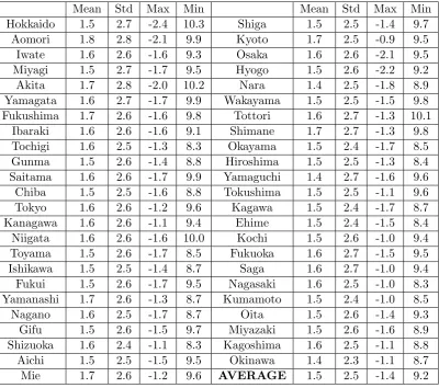
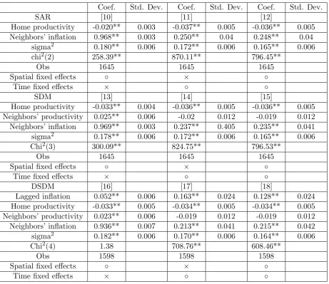
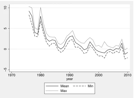
Table 1 lists inflation (All items) for the 47 regions broadly in the order of the location of the regions from north to south and suggests that all regions have experienced a relatively low inflation by international standards of around 1.5% per annum, ranging from 1.4% in Nara, Yamaguchi and Okinawa to 1.8% in Aomori. Inflation volatility in terms of standard deviations seems to be very similar among regions, ranging from 2.3 in Okinawa to 2.8 in Ao-mori and Akita. In this regard, prices seem to be most stable in Okinawa. We also plot the average, minimum and maximum regional inflation (Figure 1), showing that inflation is time-varying and reaches relatively high levels (around 10%) at times of oil shocks. In contrast, inflation has been stable and low in more recent periods when Japan underwent economic recession and deflation.
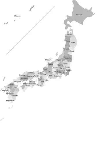
Figure 2 plots the geographical locations of each region. The geograph-ical distance (d) between regions (measured by the distance between capi-tal cities) is obtained from the Geospatial Information Authority of Japan (http://www.gsi.go.jp/KOKUJYOHO/ kenchokan.html). The distance is calculated using the Geodetic Reference System 1980(GRS80) and is sum-marized in Figure 3, which depicts the average distance between regional capitals for each region. According to this average value, Okinawa is lo-cated significantly distant from others, while Shiga is surrounded by other regions within a short distance. This distance is used to create a weight matrix for a pair of regionsiand j(i6=j and i, j= 1,· · · , N) following the standard approach (i.e., power distance weights):
w=d−θ
ij (11)
The w is a symmetric matrix and the diagonal elements are zero, and for estimation of the model each row of the weight matrix will be normalized such that the row sum ofw becomes equal to one. We shall use two different
values forθ(θ= 1 or 2) in order to check the robustness of our results to the assumption of the weight matrix.9 In the academic literature, distance is
often used as a proxy for transaction costs, but can have wider implications. For instance, a short distance between regions would mean that neighbors tend to share a similar history, economic structure and culture, and trade more with each other.
9
In addition to the abovementioned definition ofw, we also used the weight matrix on
4
Preliminary investigation of data
The standard assumptions required for spatial models are the presence of spatial autocorrelation and the stationarity of data among others; therefore, we shall conduct several tests to understand the statistical characteristics of the data. First, in order to examine the spatial independence of regional inflation, we have implemented Moran’s I test which for regions (i, j, i6=j) can be summarized as:
Moran′sI = PN
i=1
PN
j=1wij(yi−y)(y¯ j−y)¯
PN
i=1(yi−y)¯ 2
(12)
where y is a vector of regional inflation rates, and a bar indicates the average value of the corresponding variable. Like the standard correlation coefficient, Morans I statistics range from -1 to 1, and the insignificance of the statistics (i.e., Moran’sI = 0) suggests the absence of spatial autocor-relation. When regional inflation rates are positively correlated, we would expect to have positive and significant statistics from this test.
This test is conducted for not only the most comprehensive measure of CPI inflation (i.e., All items), but also sectoral inflation in order to check whether inflation in one region has been affected by developments in others or vice versa. Following the CPI classification method, 10 major sector spe-cific items are reported in this table; namely, 1) food, 2) housing, 3) fuel, light and water charges, 4) furniture and household utensils, 5) clothes and footwear, 6) medical care, 7) transportation and communication, 8) educa-tion, 9) culture and recreaeduca-tion, and 10) miscellaneous.
Since Morans I test has been developed for cross section data, we shall implement it for each year. The results show that the null hypothesis of no spatial autocorrelation is rejected in many cases, and imply the importance of spatial autocorrelation among regional inflation (Table 2).
However, the degree of spatial autocorrelation is rather sector-specific. Notably, spatial autocorrelation is strongly present in sectors in 3) fuel, light and water charges and 7) transportation and communication. In such cases, the average value of Morans I test is reported to be positive. This is an
in-dustries; since there are a limited number of supplies, these companies tend to set similar (if not the same) prices in regions nearby.10 In contrast, very
weak evidence of spatial autocorrelation is reported for economic sectors such as 4) furniture and household utensils and 6) medical care. In these in-dustries, Morans I statistics are often negative and statistically insignificant.
Table 3 examines the stationarity of regional inflation, which is required for estimation of the standard spatial models. Three panel unit root tests; namely, the Levin-Lin-Chu (LLC), Im-Pesaran-Shin (IPS) and Fisher-type ADF tests, have been implemented to examine the null hypothesis of the unit root. The alternative hypothesis differs according to the tests: while that of the LLC is that all panels are stationary, the latter two tests evaluate the alternative that some panels are stationary. In any case, all these tests lead to a conclusion against the null, and this is consistent with that the study on the European Monetary Union (EMU) (BECK et al. 2006).
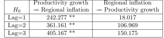
Finally, we also examine the relationship between regional inflation and its own productivity growth (Figure 4). While it is difficult to draw a clear conclusion from this figure, it appears that a negative relationship exists between these variables. This is inconsistent with theoretical predictions and shall be discussed later when interpreting our empirical results (Section 6). Furthermore, the causality tests based on the panel vector auto-regression (VAR) confirm the theoretical prediction of the BS theorem (Table 4); in other words, productivity growth results in changes in regional inflation. But no evidence is found that inflation has caused productivity growth. This ensures our a priori assumption about the exogeneity of productivity growth in our spatial econometric models which will be explained next.
5
Spatial Econometric models
The spatial econometric approach has been rapidly developed over the past decade, and today it has been applied in many areas of research (see the survey in LESAGE and PACE 2009). But as discussed in the Introduction, there are few attempts at inflation analysis probably due to the fact that inflation has often been analyzed at the national level with a presumption of equality in regional inflation. However, spatial autocorrelation is pertinent here since we relax this resumption. Furthermore, the consideration of geo-graphical space is more relevant here compared with analysis of other prices, e.g., of financial assets (stocks and bonds) since these assets can easily be
10
traded using modern technologies, and there is a less significant amount of transaction costs involved in trading compared with consumer goods, the main components of the CPI, which need to be physically shipped.
While the majority of spatial models have been designed for cross-section analysis, we use spatial panel data models which make use of time-series information. More concretely, while different types of spatial models are available, this paper uses the spatial autoregressive model (SAR) and the spatial Durbin model (SDM). However, it is the SDM which we use as the main vehicle of the research due to its proximity to the theoretical specifica-tion (9) and its appropriateness for analyzing spillover effects (VEGA and ELHORST 2013, p. 10). We present results from the SAR, the most basic spatial model, for the purposes of comparison.
For the endogenous variable (y) which consists of N(i = 1,· · · , N) re-gions and timeT(t= 1,· · · , T), the SAR can be expressed as11:
yt=ατN +µ+ξtτN +ρwyt+xtβ+et (13)
Here, yt is a N ×1 vector consisting of regional inflation, and τN is a
N×1 vector of one. Further,x is aN ×k matrix of explanatory variables (i.e., productivity), and their parameters β is a k×1 vector. The w is a spatial weight which, as mentioned in the previous section, is determined in this paper by the location of the regions. Thus our definition of wis closely associated with transaction costs: home inflation is not strongly correlated with that of distant neighbors. One interesting feature of this spatial model (13) is the inclusion of a spatially lagged variable (wyt(wyt=PN
j=1wijyjt,
wherewij is an element of the spatial weight matrix w)), which represents a
linear combination of neighbors contemporaneous inflation and thus is ∆p∗ in (9). Soρ captures the sensitivity ofytto spatially lagged variables. This is a notable advantage of the spatial model over the conventional panel data estimation models.12
Given the presence of spatial dependence (Table 2) and significant dis-crepancies between regional inflation rates (e.g., NAGAYASU 2011), we use the SAR (Eq. (13)), the most general specification of this kind due to inclu-sion of both the spatial fixed effectµ) and the time period fixed effect (ξtτN).
13 Finally, e
it is the residual (et = (u1t, u2t,· · ·, uN t)′, uit ∼N(0, σ2)). We
11
Our expression of spatial models is consistent with ELHORST (2014).
12
Otherwise, one needs to construct a neighbors variable (i.e., a variable with an asterisk in (1)) using their average with some arbitrary weights prior to the estimation.
13
expect ρ >0 following the result from Moran’s I for All items: neighbors’ inflation is positively related with inflation at home (i.e., yit). Similarly, home productivity increases its own inflation through raising wages and thusβ>0.
One potential problem in (13) is related to the endogeneity of explana-tory variables. It is fairly easy to accept that our weight matrix (w) is exogenous. However, even though productivity (x) is found to be exogenous (Table 4), OLS estimators are still biased due to the inclusion ofwytin the SAR. In other words, changes in home inflation because of neighbors infla-tion are likely to have feedback effects which then influence the neighbors inflation. In order to circumvent this bias, our estimation is based on the maximum likelihood (ML) method which corrects this bias when obtaining the residual term to carry out the ML (see ELHORST 2012).
Since the SAR is incapable of capturing the effects of neighbors pro-ductivity on home inflation, we also consider the SDM. This model is more consistent with our theoretical model and is an extension to the SAR:
yt=ατN +µ+ξtτN +ρwyt+xtβ+wxtθ+et (14)
This equation includes spatially lagged explanatory variables, wxt. In
our setting, this extra variable represents neighbors’ productivity, i.e., a∗. We expect that improvements in neighbors’ productivity will reduce home inflation and thus θ < 0; the expected sign for other parameters remains the same as in (13). The specification in which prices (inflation rates) are determined by productivity (growth) is consistent with previous studies an-alyzing the BS effect (see survey articles, e.g., SARNO and TAYLOR 2003, BAHMANI-OSKOOEE and NASIR 2005). This model is also used in the hybrid Phillips curve model (YESILYURT and ELHORST 2013), one of two previous studies which employed spatial models in regional inflation analysis.
Finally, we shall add a lagged endogenous variable (yt−1) in (14) in or-der to introduce inflation persistence. Inflation persistence is often observed worldwide and a classic explanation is ”menu costs” which prevent instan-taneous adjustments in prices in response to exogenous shocks (e.g., BANK OF JAPAN (BOJ) 2000).
yt=ατN +µ+ξtτN+τyt−1+ρwyt+xtβ+wxtθ+et (15)
statistical tests to find the best model, models (14) and (15) are congruent with our theoretical model (9). 14 In this respect, model (13) suffers from
a misspecification bias on theoretical grounds since neighbors’ productivity (a∗) is omitted. The estimation procedure for a spatial dynamic panel model is explained by LEE and YU (2010b). See also MARQUES et al. (2013) who analyzed Turkish regional inflation using the dynamic spatial model in order to introduce price inertia.
6
Empirical results
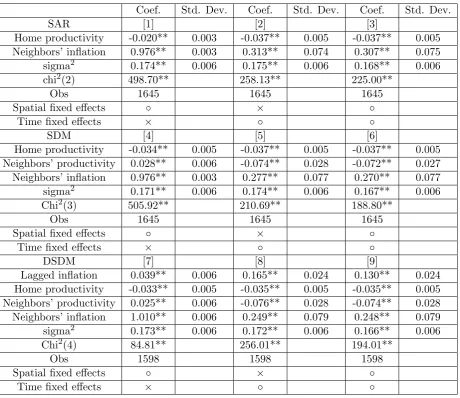
Tables 5 to 7 presents the empirical results from these spatial models applied to the most comprehensive CPI (All items) as it has been most frequently monitored by policymakers and analyzed by researchers. Tables 5 and 6 summarize parameter estimates using two different types of weight matrices (θ = 1 or 2 in Eq. (11)) to check the robustness of results to our assump-tion about the weight matrix. We generally find the results to be consistent with economic theory, confirming the BS effect, spillovers of inflation and productivity, and inflation persistence.
First, we have confirmed that neighbors’ inflation and geographical dis-tance between regions are important factors affecting regional inflation. The ρ is positive and statistically significant in all models; a rise in neighbors’ inflation tends to increase inflation at home. This result can also be inter-preted as evidence that distant neighbors do not affect home inflation very much at all. While the size of this parameter drops when the time period fixed effect is included in the model, this parameter remains significant.
Second, productivity growth is also found to have a significant effect on inflation on many occasions. In contrast to the BS prediction, productivity improvements in neighboring regions (a∗) are found to increase domestic inflation (θ > 0) when the time period fixed effect is not included. How-ever, while the statistical significance differs by the definition of the weight matrix, θ turns out to be negative (θ < 0) in the SDM and DSDM with the time period fixed effect. Since there is a tendency for regional inflation to move in a similar direction and the time period fixed effect is relevant in our data, we consider thatθ <0 is a more reliable result (see [6], [9], [15] and [18] in Tables 5 and 6).
The other productivity variable (a) is reported to enter negatively and significantly in all models, implying that technological developments at home will reduce inflation rates. This parameter sign is inconsistent with
theo-14
retical predictions, and may result from the measurement error in data. While our CPI is compiled mainly for capital cities, productivity here cov-ers economic activities in all cities and villages in regions. Therefore, home productivity in this study covers a wider spatial area than the CPI, and incudes productivity changes in cities and villages that should actually be included in those in neighboring regions. Given that there is heterogeneity between urban and rural economic developments and that productivity is higher in rural areas, i.e., capital cities (SAKAMOTO 2013), the inclusion of productivity in rural areas may have a downward bias in the parameter. Alternatively, the negative sign for a may simply reflect the excess sup-ply situation during the recent prolonged recession/deflation period; weak private consumption is a notable economic phenomenon in this period sug-gesting that productivity improvements did not lead to increases in wages (and prices).
Furthermore, the results aboutρ and θ imply that there is a significant discrepancy between regional inflation rates. Spatial models with two fixed effects generally reject equality among regional inflation (ρ = 1) and also support the significant role of productivity in explaining heterogeneity in regional inflation. Therefore, our results confirm previous results (e.g., NA-GAYASU 2011) of heterogeneous inflation across Japan.
We have also introduced the lagged endogenous variable (i.e., lagged in-flation) in the SDM, and empirical results are presented under the DSDM. While our analysis is at the regional level, as expected, we confirm inflation persistence with a positive and significant parameter for τ (Tables 5 and 6). Inflation persistence is discussed to be yielded by a number of economic factors (BOJ 2000). According to the BOJs survey, for instance, in addition to menu costs, contracts and royalties to customers and business partners are reported to have prevented instantaneous adjustments in prices in re-sponse to exogenous shocks. Similarly, CRUCINI et al. (2010) consider both price persistence and geographical distance in explaining variations in het-erogeneity in Japanese regional prices. Further, CHOI and MATSUBARA (2007) document the persistence of relative prices in Japan, and argue that it is attributable to the market structure and the tradability of goods. The persistence in regional inflation is also consistent with experiences in other countries, e.g., the euro area (BECK et al. 2006), Italy (VAONA and AS-CARI 2012) and Korea (TILLMANN 2013). Note that our analysis based on a fixed effects model (as opposed to random effects model) is supported by the Hausman test (Chi2 in Tables 5 and 6).
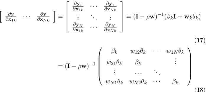
other regions affects home inflation. Thus the indirect effect can be consid-ered as a spillover. It is essential to calculate these effects since, as LESAGE and PACE (2009) have explained, the parameters in Tables 5 and 6 do not present precise information about the effects of explanatory variables due to the presence of spatially lagged variables. In this connection, one needs to consider the mutual influences of regional inflation, and presentation of these effects has become the standard format in spatial analysis. These effects can be seen by rewriting (15) as:
yt= (I−ρw)−1τyt−1+ (I−ρw)−1(xtβ+wxtθ) +ǫ (16)
whereǫt=ατN+µ+ξtτN+et, andIis an identity matrix. Our focus is
on productivity and thus the second component on the right hand side. The sensitivity of y with respect to the kth element in x can then be expressed using the partial derivative of (16):
h
∂y ∂x1k · · ·
∂y ∂xN k
i = ∂y1
∂x1k · · ·
∂y1
∂xN k ..
. . .. ...
∂yN
∂x1k · · ·
∂yN
∂xN k
= (I−ρw)−1(β
kI+wkθk)
(17)
= (I−ρw)−1
βk w12θk · · · w1Nθk
w21θk βk ...
..
. · · · . ..
wN1θk wN2θk · · · βk
(18)
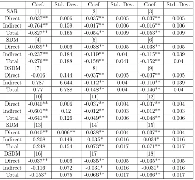
The direct effect is calculated as the average of the diagonal elements of the matrix, and the indirect effect as the row sums of the off-diagonal elements of the matrix.15 As can be seen from (17), off-diagonal elements
[image:15.595.128.477.359.515.2]in the parentheses become zero when θ = 0 and/or w= 0. Thus the SDM and DSDM offer a more general framework to analyze spillovers compared with the SAR which assumesθ = 0 from the outset. Finally, the total effect becomes equal to the sum of the direct and indirect effects.
Table 7 summarizes estimates of the total, direct and indirect effects, and suggests that both direct and indirect effects are important for under-standing regional inflation. All parameters are negative which is consistent
15
with our estimates for this variable in Tables 5 and 6 with two fixed ef-fects. Furthermore, there is evidence from the SDM and DSDM that the indirect (i.e., spillover) effect is nonnegligible, confirming the close economic relationship between regions in Japan. Since the first stage estimation (i.e., Tables 5 and 6) did not calculate the standard errors without distinguishing between these effects, the inferences of these effects are obtained by simula-tions (1,000 replicasimula-tions) following LESAGE and PACE (2009) in order to evaluate separately the significance of these effects.
7
Conclusion
This paper analyzes heterogeneity in regional inflation in Japan. Unlike previous empirical studies, we consider both the Balassa-Samuelson (BS) effect and the geographical locations of regions which are often regarded as theoretically reasons for heterogeneity in regional inflation. Furthermore, in order to capture these effects, we employ spatial econometric models which have been developed rapidly over recent years but have rarely been applied in inflation analysis.
In short, we have provided further evidence of heterogeneity in regional inflation in Japan and confirmed that it can be explained by the spatial lo-cations of regions and by productivity growth. In particular, inflation in one region is closely associated with developments in neighbors inflation and pro-ductivity, consistent with the BS effect. Finally, inflation inertia, which has been observed in the national level data, is present in regional data as well. This result is also in line with regional inflation analysis in other countries (e.g., YESILYURT and ELHORST 2013). Thus, our findings imply that heterogeneous inflation in Japan is caused by productivity and transaction costs, and complements previous studies (NAGAYASU 2011, KANO et al. 2013) that have provided empirical evidence of heterogeneous price/inflation from Japanese regional data but which considered only the transaction costs.
References
[1] ALTISSIMO F., EHRMANN M. and SMETS F. (2006) Inflation per-sistence and price-setting behavior in the euro area: a summary of the IPN evidence, European Central Bank Occasional Paper Series No. 46.
[2] BANK OF JAPAN (2000) Nihon kigyo no kakaku settei kodo, Tokyo: Bank of Japan.
[3] BALASSA, B. (1964) The purchasing power parity doctrine: a reap-praisal, Journal of Political Economy 72 (6), 584?596.
[4] BAHMANI-OSKOOEE, M. and NASIR A.B.M. (2005) Productivity bias hypothesis and the purchasing power parity: a review article, Jour-nal of Economic Surveys 19, 672-696.
[5] BECK G W., HUBRICH K., and MARCELLIONO M. (2006) Regional inflation dynamics within and across euro area countries and a compar-ison with the US, European Central Bank Working Paper Series No. 681.
[6] BUSETTI F., FABIANI S. and HARVEY A. (2006) Convergence of prices and rates of inflation, Oxford Bulletin of Economics and Statistics 68, 863-877.
[7] CASSEL G. (1918) Abnormal deviations in international exchanges, Economic Journal 28(112), 413?415.
[8] CEGLOWSKI, J. (2003) The law of one price: intranational evidence for Canada, Canadian Journal of Economics 36(2), 373-400.
[9] CHEN N. (2004) The behavior of relative prices in the European Union: a sectoral analysis 48, 1257-1286.
[10] CHOI, C-Y., and MATSUBARA, K. (2007) Heterogeneity in the per-sistence of relative prices: what do the Japanese cities tell us? Journal of the Japanese and International Economies 21, 260-286.
[11] CRUCINI, M.J., SHINTANI, M., and TSURUGA, T. (2010) The law of one price without the border: the role of distance versus sticky prices, Economic Journal 120, 462-480.
[12] DE HAAN J. (2010) Inflation differentials in the euro area: a survey, in The European Central Bank at Ten, J.de Haan and H. Berger (eds.) Berlin: Springer-Verlag.
[14] ELHORST J. P. (2012) Matlab software for spatial panels, International Regional Science Review. DOI: 10.1177/0160017612452429.
[15] ELHORST J. P. (2014) Spatial Econometrics: from Cross-sectional Data to Spatial Panels, London: Springer.
[16] ENGEL C., and ROGERS J H. (1996) How wide is the border? Amer-ican Economic Review 86, 1112-1125.
[17] ESAKA T. (2003) Panel unit root tests of purchasing power parity between Japanese cities, 1960-1998: disaggregated price data, Japan and the World Economy 15, 233-244.
[18] EUROPEAN CENTRAL BANK (2003) Inflation differentials in the euro area: potential causes and policy implications, Frankfurt: ECB.
[19] IKENO, H. (2014) Pairwise tests of convergence of Japanese local price levels, International Review of Economics and Finance 31, 232-248.
[20] KANO K., KANO T., and TAKECHI K. (2013) Exaggerated death of distance: revisiting distance effects on regional price dispersions, Journal of International Economics 90, 403-413.
[21] LEE L-F., and YU J. (2010a) Estimation of spatial autoregressive panel data models with fixed effects, Journal of Econometrics 157, 53-67.
[22] LEE L-F., and YU, J. (2010b) A spatial dynamic panel data model with both time and individual fixed effects, Econometric Theory 26, 564-597.
[23] LESAGE J., and PACE R. K. (2009) Introduction to Spatial Econo-metrics, London: CRC Press.
[24] LOPEZ C., and PAPELL D. H. (2012) Convergence of euro area infla-tion rates, Journal of Internainfla-tional Money and Finance 31, 1440-1458.
[25] MARQUES H., PINO G., and HORRILLO J. D. D. T. (2013) Regional inflation dynamics using space-time models, Empirical Economics (pub-lished online).
[26] MUNDELL R. A. (1961) A theory of optimum currency areas, Ameri-can Economic Review 51, 657?665.
[27] NAGAYASU J. (2011) Heterogeneity and convergence of regional infla-tion (prices), Journal of Macroeconomics 33, 711-723.
[29] NAGAYASU J., and LIU Y. (2008) Relative prices and wages in China: evidence from a panel of provincial data, Journal of Economic Integra-tion 23, 183-203.
[30] PARSLEY, D. C., and WEI S-J. (1996) Convergence to the law of one price without trade barriers or currency fluctuations, Quarterly Journal of Economics 111, 1211-1236.
[31] PIRAS G., and PRUCHA I. R. (2013) Finite sample properties of pre-test estimators of spatial models. Regional Science and Urban Eco-nomics 46, 103-115.
[32] RABANAL R. (2009) Inflation differentials between Span and the EMU: a DSGE perspective, Journal of Money, Credit and Banking 41, 1141-1166.
[33] SAKAMOTO, H. (2013) Intra-regional disparity and municipal merger: case study in Fukuoka prefecture, ICEAD, Japan.
[34] SAMUELSON P. A. (1964) Theoretical notes on trade problems, Re-view of Economics and Statistics 46(2), 145?154.
[35] SARNO L. and TAYLOR M. P. (2003) The Economics of Exchange Rates. Cambridge: Cambridge University Press.
[36] TILLMANN P. (2013) Inflation targeting and regional inflation persis-tence: evidence from Korea, Pacific Economic Review 18, 147-161.
[37] VAONA, A. (2010) Intra-national purchasing power parity and Balassa-Samuelson effects in Italy, Economics Department, University of Verona WP No. 12.
[38] VAONA, A., and ASCARI, G. (2012) Regional inflation persistence: evidence from Italy, Regional Studies 46, 509-523.
[39] VEGA S. H., and ELHORST J. P. (2013) On spatial economic models, spillover effects and W. http://www-sre.wu.ac.at/ersa/ersaconfs/ersa13/ERSA2013 paper 00222.pdf .
Table 1: Summary statistics of regional inflation (%)
Mean Std Max Min Mean Std Max Min Hokkaido 1.5 2.7 -2.4 10.3 Shiga 1.5 2.5 -1.4 9.7
Aomori 1.8 2.8 -2.1 9.9 Kyoto 1.7 2.5 -0.9 9.5 Iwate 1.6 2.6 -1.6 9.3 Osaka 1.6 2.6 -2.1 9.5 Miyagi 1.5 2.7 -1.7 9.5 Hyogo 1.5 2.6 -2.2 9.2 Akita 1.7 2.8 -2.0 10.2 Nara 1.4 2.5 -1.8 8.9 Yamagata 1.6 2.7 -1.7 9.9 Wakayama 1.5 2.5 -1.5 9.8 Fukushima 1.7 2.6 -1.6 9.8 Tottori 1.6 2.7 -1.3 10.1
Table 2: Moran’sI tests Y ea r A ll it em s F o o d (2 ) H o u si n g (1 5 ) F u el , li g h t a n d w a te r ch a rg es (1 8 ) F u rn it u re a n d h o u se h o ld u te n si ls (2 3 ) C lo th es a n d fo o tw ea r (3 1 ) M ed ic a l ca re (4 0 ) T ra n sp o rt a ti o n a n d co m m u n ic a ti o n (4 4 ) E d u ca ti o n (4 8 ) C u lt u re a n d re cre a ti o n (5 2 ) M is ce ll a n eo u s (5 7 ) p-values
1976 0.005 0.240 0.080 0.040 0.245 0.311 0.249 0.000 0.426 0.022 0.000
1977 0.001 0.000 0.000 0.002 0.203 0.136 0.108 0.011 0.124 0.057 0.183
1978 0.001 0.000 0.378 0.289 0.265 0.038 0.021 0.316 0.330 0.178 0.185
1979 0.229 0.113 0.303 0.000 0.245 0.201 0.495 0.376 0.495 0.388 0.048
1980 0.002 0.001 0.033 0.000 0.196 0.261 0.236 0.000 0.099 0.312 0.210
1981 0.009 0.000 0.221 0.002 0.498 0.142 0.137 0.000 0.351 0.053 0.379
1982 0.000 0.003 0.319 0.000 0.313 0.420 0.392 0.162 0.064 0.427 0.277
1983 0.445 0.406 0.307 0.089 0.376 0.297 0.454 0.045 0.144 0.339 0.049
1984 0.486 0.115 0.392 0.006 0.252 0.086 0.430 0.002 0.207 0.001 0.246
1985 0.283 0.344 0.280 0.003 0.368 0.102 0.129 0.022 0.376 0.251 0.256
1986 0.275 0.089 0.349 0.000 0.417 0.272 0.336 0.073 0.255 0.425 0.138
1987 0.296 0.399 0.336 0.007 0.325 0.426 0.219 0.000 0.200 0.309 0.060
1988 0.000 0.000 0.065 0.000 0.352 0.482 0.141 0.025 0.216 0.074 0.342
1989 0.008 0.277 0.002 0.001 0.357 0.316 0.012 0.409 0.394 0.295 0.414
1990 0.074 0.001 0.002 0.000 0.125 0.473 0.326 0.122 0.374 0.117 0.363
1991 0.117 0.001 0.013 0.002 0.367 0.003 0.448 0.051 0.316 0.192 0.094
1992 0.000 0.335 0.022 0.013 0.361 0.479 0.195 0.000 0.401 0.241 0.403
1993 0.155 0.000 0.024 0.012 0.087 0.040 0.434 0.163 0.424 0.307 0.384
1994 0.028 0.004 0.489 0.258 0.285 0.448 0.292 0.035 0.215 0.161 0.007
1995 0.415 0.069 0.309 0.461 0.386 0.232 0.211 0.001 0.439 0.121 0.426
1996 0.044 0.258 0.040 0.001 0.060 0.286 0.253 0.000 0.440 0.014 0.370
1997 0.049 0.044 0.220 0.222 0.187 0.226 0.243 0.482 0.394 0.349 0.442
1998 0.176 0.395 0.190 0.000 0.106 0.318 0.385 0.002 0.350 0.121 0.122
1999 0.230 0.000 0.280 0.353 0.335 0.464 0.405 0.000 0.369 0.006 0.240
2000 0.050 0.037 0.316 0.000 0.363 0.456 0.077 0.023 0.292 0.416 0.161
2001 0.253 0.240 0.296 0.029 0.200 0.371 0.210 0.385 0.360 0.018 0.032
2002 0.480 0.145 0.039 0.000 0.333 0.039 0.446 0.471 0.106 0.277 0.300
2003 0.148 0.276 0.357 0.000 0.053 0.337 0.001 0.293 0.414 0.181 0.068
2004 0.088 0.369 0.161 0.000 0.073 0.453 0.335 0.214 0.184 0.248 0.199
2005 0.069 0.225 0.332 0.000 0.043 0.481 0.081 0.005 0.027 0.143 0.362
2006 0.118 0.104 0.233 0.000 0.286 0.463 0.090 0.005 0.459 0.426 0.331
2007 0.017 0.107 0.443 0.007 0.201 0.189 0.217 0.317 0.456 0.475 0.388
2008 0.082 0.129 0.366 0.000 0.433 0.100 0.470 0.000 0.158 0.014 0.297
2009 0.000 0.009 0.494 0.000 0.488 0.189 0.196 0.000 0.377 0.430 0.438
2010 0.403 0.264 0.046 0.000 0.472 0.420 0.140 0.001 0.000 0.158 0.178
Ave.
Note: The numbers in parentheses indicate the code numbers for data classi-fication used by the Ministry of Internal Affairs and Communication. Statis-tics significant at the 5% level are marked in bold.
Table 3: The stationarity of regional inflation
LLC IPS Fisher-ADF All items −15.3064∗∗ −18.3617∗∗ 795.4853∗∗
Food (2) −19.7453∗∗ −22.8192∗∗ 954.2189∗∗ Housing (15) −17.7332∗∗ −20.3622∗∗ 869.1275∗∗ Fuel, light and water charges (18) −17.6268∗∗ −22.5343∗∗ 944.3937∗∗ Furniture and household utensils (23) −15.6058∗∗ −18.6328∗∗ 811.5773∗∗ Clothes and footwear (31) −21.2889∗∗ −24.4985∗∗ 1013.8402∗∗
Medical care (40) −19.4160∗∗ −23.6366∗∗ 984.0173∗∗ Transportation and communication (44) −18.4106∗∗ −24.7262∗∗ 1021.9635∗∗
Education (48) −12.8192∗∗ −17.6173∗∗ 775.2560∗∗ Culture and recreation (52) −16.8591∗∗ −20.0646∗∗ 859.5731∗∗ Miscellaneous (57) −17.3087∗∗ −21.5294∗∗ 910.4215∗∗
Table 4: Panel Granger non-causality test between regional inflation and productivity growth
H0
Productivity growth 9 Regional inflation
Regional inflation 9Productivity growth Lag=1 242.277 ** 18.017
Lag=2 361.161 ** 106.969 Lag=3 405.167 ** 150.175
Table 5: Results from the panel spatial econometric models (θ= 1)
Coef. Std. Dev. Coef. Std. Dev. Coef. Std. Dev.
SAR [1] [2] [3]
Home productivity -0.020** 0.003 -0.037** 0.005 -0.037** 0.005 Neighbors’ inflation 0.976** 0.003 0.313** 0.074 0.307** 0.075 sigma2 0.174** 0.006 0.175** 0.006 0.168** 0.006
chi2(2) 498.70** 258.13** 225.00**
Obs 1645 1645 1645
Spatial fixed effects ◦ × ◦
Time fixed effects × ◦ ◦
SDM [4] [5] [6]
Home productivity -0.034** 0.005 -0.037** 0.005 -0.037** 0.005 Neighbors’ productivity 0.028** 0.006 -0.074** 0.028 -0.072** 0.027 Neighbors’ inflation 0.976** 0.003 0.277** 0.077 0.270** 0.077 sigma2 0.171** 0.006 0.174** 0.006 0.167** 0.006
Chi2(3) 505.92** 210.69** 188.80**
Obs 1645 1645 1645
Spatial fixed effects ◦ × ◦
Time fixed effects × ◦ ◦
DSDM [7] [8] [9]
Lagged inflation 0.039** 0.006 0.165** 0.024 0.130** 0.024 Home productivity -0.033** 0.005 -0.035** 0.005 -0.035** 0.005 Neighbors’ productivity 0.025** 0.006 -0.076** 0.028 -0.074** 0.028 Neighbors’ inflation 1.010** 0.006 0.249** 0.079 0.248** 0.079 sigma2 0.173** 0.006 0.172** 0.006 0.166** 0.006
Chi2(4) 84.81** 256.01** 194.01**
Obs 1598 1598 1598
Spatial fixed effects ◦ × ◦
Time fixed effects × ◦ ◦
Table 6: Results from the panel spatial econometric models (θ= 2)
Coef. Std. Dev. Coef. Std. Dev. Coef. Std. Dev.
SAR [10] [11] [12]
Home productivity -0.020** 0.003 -0.037** 0.005 -0.036** 0.005 Neighbors’ inflation 0.968** 0.003 0.250** 0.04 0.248** 0.04
sigma2 0.180** 0.006 0.172** 0.006 0.165** 0.006
chi2(2) 258.39** 870.11** 796.45**
Obs 1645 1645 1645
Spatial fixed effects ◦ × ◦
Time fixed effects × ◦ ◦
SDM [13] [14] [15]
Home productivity -0.033** 0.004 -0.036** 0.005 -0.036** 0.005 Neighbors’ productivity 0.025** 0.006 -0.02 0.012 -0.019 0.012 Neighbors’ inflation 0.969** 0.003 0.237** 0.405 0.235** 0.041 sigma2 0.178** 0.006 0.172** 0.006 0.165** 0.006
Chi2(3) 300.09** 824.75** 796.53**
Obs 1645 1645 1645
Spatial fixed effects ◦ × ◦
Time fixed effects × ◦ ◦
DSDM [16] [17] [18]
Lagged inflation 0.052** 0.006 0.163** 0.024 0.128** 0.024 Home productivity -0.033** 0.005 -0.034** 0.005 -0.034** 0.005 Neighbors’ productivity 0.023** 0.006 -0.019 0.012 -0.019 0.012 Neighbors’ inflation 0.936** 0.007 0.213** 0.041 0.215** 0.042 sigma2 0.182** 0.006 0.170** 0.006 0.164** 0.006
Chi2(4) 1.38 708.76** 608.46**
Obs 1598 1598 1598
Spatial fixed effects ◦ × ◦
Time fixed effects × ◦ ◦
Table 7: Total, direct and indirect effects of changes in home productivity
Coef. Std. Dev. Coef. Std. Dev. Coef. Std. Dev.
SAR [1] [2] [3]
Direct -0.037** 0.006 -0.037** 0.005 -0.037** 0.005 Indirect -0.764** 0.159 -0.017** 0.006 -0.016** 0.006 Total -0.827** 0.165 -0.054** 0.009 -0.053** 0.009
SDM [4] [5] [6]
Direct -0.039** 0.006 -0.038** 0.005 -0.038** 0.005 Indirect -0.237** 0.184 -0.119** 0.04 -0.115** 0.039 Total -0.276** 0.188 -0.158** 0.041 -0.152** 0.04
DSDM [7] [8] [9]
Direct -0.016 0.144 -0.037** 0.005 -0.037** 0.005 Indirect 0.787 6.644 -0.112** 0.04 -0.110** 0.039 Total 0.77 6.788 -0.148** 0.04 -0.146** 0.04
[10] [11] [12]
Direct -0.040** 0.006 -0.037** 0.004 -0.037** 0.004 Indirect -0.601** 0.12 -0.012** 0.003 -0.012** 0.003 Total -0.641** 0.126 -0.049** 0.006 -0.048** 0.006
SDM [13] [14] [15]
Direct -0.040** 0.006** -0.038** 0.004 -0.037** 0.004 Indirect -0.208 0.149 -0.035* 0.016 -0.034* 0.016 Total -0.248 0.154 -0.073** 0.017 -0.071** 0.017
DSDM [16] [17] [18]
Direct -0.037** 0.006 -0.035** 0.005 -0.035** 0.005 Indirect -0.116 0.072 -0.031* 0.016 -0.031* 0.016 Total -0.153* 0.075 -0.066** 0.017 -0.066** 0.017
Figure 1: Average, minimum, and maximum regional inflation rates (%)
−5
0
5
10
1970 1980 1990 2000 2010
year
Mean Min
Max
Figure 4: Regional inflation vs Productivity growth per employer
−5
0
5
10
Inflation (%)
−10 0 10 20