Flexible distribution modeling with the generalized lambda distribution

Munich Personal RePEc Archive

Flexible distribution modeling with the

generalized lambda distribution

Chalabi, Yohan and Scott, David J and Wuertz, Diethelm

November 2012

Online at

https://mpra.ub.uni-muenchen.de/43333/

Flexible Distribution Modeling with the

Generalized Lambda Distribution

Yohan Chalabi

_{Diethelm Wuertz}

Institute for Theoretical Physics, ETH Zurich, Switzerland

Computational Science and Engineering, ETH Zurich, Switzerland

David J. Scott

Department of Statistics, University of Auckland, New Zealand

November 2012

We consider the use of the generalized lambda distribution (GLD) family as a flexible distribution with which to model financial data sets. The GLD can assume distributions with a large range of shapes. Analysts can therefore work with a single distribution to model almost any class of financial assets, rather than needing several. This becomes especially useful in the estimation of risk measures, where the choice of the distribution is crucial for accuracy. We introduce a new parameterization of the GLD, wherein the location and scale parameters are directly expressed as the median and interquartile range of the distribution. The two remaining parameters characterize the asymmetry and steepness of the distribution. Conditions are given for the existence of its moments, and for it to have the appropriate support. The tail behavior is also studied. The new parameterization brings a clearer interpretation of the parameters, whereby the distribution’s asymmetry can be more readily distinguished from its steepness. This is in contrast to current parameterizations of the GLD, where the asymmetry and steepness are simultaneously described by a combination of the tail indices. Moreover, the new parameterization can be used to compare data sets in a convenient asymmetry and steepness shape plot.

∗_{Corresponding author. Email address: [email protected]. Postal address: Institut für Theoretische Physik,}

Keywords Quantile distributions_·Generalized lambda distribution _·Shape plot representation

JEL Classification C16 _·C13

1 Introduction

It is well known that distributions of financial returns can exhibit heavy-tails, skewness, or both. This trait is often taken as stylized fact, and can be modeled byα-stable distributions. The drawback to using these distributions is that they do not all have closed form for their densities and distribution functions. In this regard, the generalized lambda distribution (GLD) offers an alternative. The four-parameter GLD family is known for its high flexibility. It can create distributions with a large range of different shapes. It shares the heavy-tail and skewness properties of theα-stable distribution. Excepting Corrado [2001] and Tarsitano [2004], there has been little application of the GLD to financial matters. However, as will be covered in this chapter, the shape range of the GLD family is so large that it can accommodate almost any financial time series. Analysts can therefore work with a single distribution, rather than needing several. This becomes especially useful in the estimation of risk measures, where the choice of the distribution is crucial for accuracy. Furthermore, the GLD is defined by a quantile function. Its parameters can be estimated even when its moments do not exist.

This paper introduces a more intuitive parameterization of the GLD that expresses the location and scale parameters directly as the median and interquartile range of the distribution. The two remaining shape parameters respectively characterize the asymmetry and steepness of the distribution. This is in contrast to the standard parameterization, where the asymmetry and steepness are described by a combination of the two tail indices. In Section 2 we review the history of the generalized lambda distribution. Then, in Section 3, the new formulation is derived, along with the conditions of the various distribution shape regions and the moment conditions.

Applications of the new GLD parameterization are presented in Section 5. First, the new parameterization is used to compare data sets in a convenient asymmetry and steepness shape plot. The use of the asymmetry and steepness shape plot is illustrated by comparing equities returns from the NASDAQ-100 stock index. Second, widely used financial risk measures, such as the value-at-risk and expected shortfall, are calculated for the GLD. Third, the shape plot is used to illustrated the apparent scaling law and self-similarity of high frequency returns.

2 The generalized lambda distribution

The GLD is an extension of Tukey’s lambda distribution [Hastings et al., 1947; Tukey, 1960, 1962]. Tukey’s lambda distribution is symmetric and is defined by its quantile function. It was introduced to efficiently redistribute uniform random variates into approximations of other distributions [Tukey, 1960; Van Dyke, 1961]. Soon after the introduction of Tukey’s lambda distribution, Hogben [1963], Shapiro et al. [1968], Shapiro and Wilk [1965], and Filliben [1975] introduced the non-symmetric case in sampling studies. Over the years, Tukey’s lambda distribution became a versatile distribution, with location, scale, and shape parameters, that could accommodate a large range of distribution forms. It gained use as a data analysis tool and was no longer restricted to approximating other distributions. Figure 1 illustrates the four qualitatively different shapes of the GLD: unimodal, U-shaped, monotone and S-shaped. The GLD has been applied to numerous fields, including option pricing as a fast generator of financial prices [Corrado, 2001], and in fitting income data [Tarsitano, 2004]. It has also been used in meteorology [Ozturk and Dale, 1982], in studying the fatigue lifetime prediction of materials [Bigerelle et al., 2006], in simulations of queue systems [Dengiz, 1988], in corrosion studies [Najjar et al., 2003], in independent component analysis [Karvanen et al., 2000], and in statistical process control [Pal, 2004; Negiz and Çinar, 1997; Fournier et al., 2006].

The parameterization of the extended Tukey’s lambda distributions has a long history of development. Contemporary parameterizations are those of Ramberg and Schmeiser [1974] and Freimer et al. [1988]. Ramberg and Schmeiser [1974] generalized the Tukey lambda distribution to four parameters called the RS parameterization:

QRS(u) =λ1+

1

λ2 h

uλ3 _−(1−u)λ4i_{, (1)}

where QRS = F

−1

RS is the quantile function for probabilities u, λ1 is the location parameter,

λ2 is the scale parameter, and λ3 and λ4 are the shape parameters. In order to have a valid

distribution function where the probability density functionf is positive for allx and integrates to one over the allowed domain, i.e.,

f(x)_≥0 and

Z Q(1)

Q(0)

Unimodal U−shape

Monotone S−shape

GLD Range of Shapes

Region λ2 λ3 λ4 Q(0) Q(1)

1 <0

≤ −1 ≥1

−∞ λ1+ (1/λ2)

  

−1< λ3<0andλ4>1

(1−λ3)

1₋λ3_(λ 4−1)

λ4−1

(λ4−λ3)λ4−λ3 =

−λ3

λ4

2 <0

≥1 ≤ −1

λ1−(1/λ2) ∞

  

λ3>1 ∧ −1< λ4<0

(1−λ4)

1₋λ₄

(λ3−1)

λ₃₋1

(λ3−λ4)λ3−λ4 =

−λ4

λ3

3 >0

>0 >0 λ1−(1/λ2) λ1+ (1/λ2)

= 0 >0 λ1 λ1+ (1/λ2)

>0 = 0 λ1−(1/λ2) λ1

4 <0

<0 <0 −∞ ∞

= 0 <0 λ1 ∞

<0 = 0 −∞ λ1

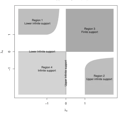
Table 1: Support regions of the GLD and conditions on the parameters given by the RS parameterization to define a valid distribution function (Karian and Dudewicz [2000]). The support regions are displayed in Fig. 2. Note that there are no conditions onλ1 to

obtain a valid distribution.

the RS parameterization has complex constraints on the parameters and support regions as summarized in Table 1 and Fig. 2.

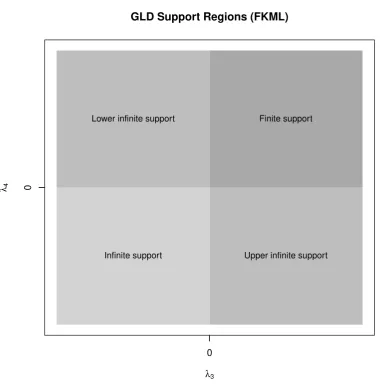
Later, Freimer et al. [1988] introduced a new parameterization called FKML to circumvent the constraints on the RS parameter values. It is expressed as

QFKML(u) =λ1+

1

λ2 "

uλ3 ₋₁

λ3 −

(1₋u)λ4 −1

λ4

#

. (2)

As in the previous parameterization, λ1 and λ2 are the location and scale parameters, andλ3

andλ4 are the tail index parameters. The advantage over the previous parameterization is that

the only constraint on the parameters is thatλ2 must be positive. Figure 3 displays the support

regions of the GLD in the FKML parameterization.

−1 0 1

−1

0

1

GLD Support Regions (RS)

λ3

λ4

Region 1 Lower infinite support

Region 3 Finite support

Region 2 Upper infinite support Region 4

Infinite support

Upper Infinite suppor

t

Lower Infinite support

0

0

GLD Support Regions (FKML)

λ3

λ4

Finite support Lower infinite support

Upper infinite support Infinite support

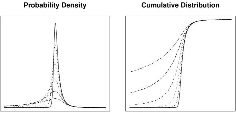
Probability Density Cumulative Distribution

Figure 4: Probability density and cumulative distribution functions for the GLD in the RS parameterization. The location and scale parameters are, λ1 = 0 and λ2 = −1,

respectively. The right tail index is fixed at λ4 = −1/4 and the left tail index, λ3,

varies in the range_{−1/16,₋1/8,₋1/4,₋1/2,₋1,₋2_}.

order statistics [Ozturk and Dale, 1985] and with percentiles [Karian and Dudewicz, 1999, 2000; Fournier et al., 2007; King and MacGillivray, 2007; Karian and Dudewicz, 2003]; the methods of moments [Ozturk and Dale, 1982; Gilchrist, 2000], L-moments [Gilchrist, 2000; Karvanen and Nuutinen, 2008], and trimmed L-moments [Asquith, 2007]; and the goodness-of-fit method with histograms [Su, 2005] and with maximum likelihood estimation [Su, 2007]. On the other side, stochastic methods have been introduced with various estimators such as goodness-of-fit [Lakhany and Mausser, 2000] or the starship method [King and MacGillivray, 1999]. Moreover, Shore [2007] studied theL2-norm estimator that minimizes the density function distance and the use of nonlinear regression applied to a sample of exact quantile values.

As noted by Gilchrist [2000], one of the criticisms of the GLD is that its skewness is expressed in terms of both tail indicesλ3 andλ4 in Eqs. (1) and (2). In one approach addressing this

concern, a five-parameter GLD was introduced by Joiner and Rosenblatt [1971], which, expressed in the FKML parameterization, can be written as,

QJR(u) =λ1+

1 2λ2

"

(1₋λ5)

uλ3 ₋₁

λ3 −

(1 +λ5)

(1₋u)λ4 −1

λ4

#

.

It has a location parameterλ1, a scale parameter λ2, and an asymmetry parameter, λ5, which

weights each side of the distribution and the two tail indices, λ3 andλ4. The conditions on

the parameters areλ2 >0and −1< λ5 <1. However, the additional parameter can make the

3 A shape parameterization of the GLD

In this chapter, it is shown how the four-parameter GLD of Eq. (2) can be transformed in terms of an asymmetry and steepness parameter without adding a new variable. Moreover, the location and scale parameters are reformulated in terms of quantile statistics. The median is used as the location parameter, and the interquartile range is used as the scale parameter.

The new parameterization brings a clearer interpretation of the parameters, whereby the asymmetry of the distribution can be more readily distinguished from the steepness of the distribution. This is in contrast to the RS and FKML parameterizations, where the asymmetry is described by a combination of the tail indices. The new formulation allows for relaxed constraints upon the support regions, and for the existence of moments for the GLD.

Another advantage of the new parameterization is that the estimation of the parameters for an empirical data set can be reduced to a two-step estimation problem, because the location and scale parameters can be directly estimated by their robust sample estimators. Note that sample quantiles can always be estimated, even when moments of the distribution do not exist. The two shape parameters can then be estimated by one of the usual estimation methods, such as the maximum likelihood estimator.

The remainder of this chapter is organized as follows. In Section 3.1, the new asymmetry-steepness parameterization of the GLD is introduced. In Section 3.2, the support of the distribution is derived in terms of its parameters, and the different support regions are illustrated in a shape plot. Then, in Section 3.3, conditions are given for the existence of its moments, and a shape plot representation is made. In Section 3.4, the tail behavior of the GLD in the new parameterization is studied. Based on the support and moment existence conditions, Section 3.5 studies the different shape regions of the distribution. Section 3.6 lists sets of parameter values that make the GLD a good approximation for several well-known distributions.

3.1 An asymmetry-steepness parameterization

In the following section, the new parameterization is expressed in the FKML form. Consider the GLD quantile function:

Q(u) =λ1+ 1

λ2

S(u_|λ3, λ4), (3)

where

S(u_|λ3, λ4) =               

ln(u)₋ln(1₋u) if λ3 = 0, λ4= 0, ln(u)_−λ1

4 h

(1₋u)λ4 ₋₁i _{if λ}

3 = 0, λ46= 0, 1

λ3 u

λ3_{−1−ln(1−u) if λ}

3 6= 0, λ4= 0, 1

λ3 u

λ3₋₁₋ 1

λ4 h

(1₋u)λ4

−1i otherwise,

for0 < u <1. Q is the quantile function for probabilities u; λ1 and λ2 are the location and

scale parameters; andλ3 andλ4 are the shape parameters jointly related to the strengths of the

lower and upper tails. In the limiting caseu= 0:

S(0_|λ3, λ4) =   

−λ13 if λ3 >0, −∞ otherwise.

In the limiting caseu= 1:

S(1_|λ3, λ4) =    1

λ4 if λ4>0, ∞ otherwise.

The median,µ˜, and the interquartile range,σ˜, can now be used to represent the location and scale parameters. These are defined by

˜

µ=Q(1/2), (5a)

˜

σ =Q(3/4)₋Q(1/4). (5b) The parametersλ1 andλ2 in Eq. (4) can therefore be expressed in terms of the median and

interquartile range as

λ1= ˜µ− 1

λ2

S(1

2|λ3, λ4),

λ2= 1 ˜

σ

S(3

4|λ3, λ4)−S( 1

4|λ3, λ4)

.

As mentioned in the introduction, one of the criticisms of the GLD is that the asymmetry and steepness of the distribution are both dependent upon both of the tail indices, λ3 and

λ4. The main idea in this chapter is to use distinct shape parameters for the asymmetry and

steepness. First, it is clear, from the definition of the GLD in Eq. (3), that when the tail indices are equal, the distribution is symmetric. Increasing one tail index then produces an asymmetric distribution. Second, the steepness of the distribution is related to the size of both tail indices: increasing both tail indices results in a distribution with thinner tails. Now, formulate an asymmetry parameter, χ, proportional to the difference between the two tail indices, and a steepness parameter,ξ, proportional to the sum of both tail indices. The remaining step is to map the unbounded interval of(λ3−λ4) to the interval(−1,1), and (λ3+λ4) to the interval (0,1). To achieve this, we use the transformation

y= _√ x

1 +x2 ↔ x=

y

p

1₋y2 wherey∈(−1,1)andx∈(−∞,∞).

The asymmetry parameter, χ, and the steepness parameter, ξ, can then be expressed as

χ= q λ3−λ4

1 + (λ3−λ4)2

, (6a)

ξ= 1 2 −

λ3+λ4 2

q

1 + (λ3+λ4)2

where the respective domains of the shape parameters are χ_∈ (₋1,1) andξ _∈(0,1). When

χis equal to 0, the distribution is symmetric. When χ is positive (negative), the distribution is positively (negatively) skewed. Moreover, the GLD becomes steeper whenξ increases. The parameterization ofχ and ξ in Eq. (6), yields a system of two equations for the tail indices λ3

andλ4:

λ3−λ4 = p χ 1₋χ2,

λ3+λ4 = 1 2−ξ p

ξ(1₋ξ).

This gives

λ3 =α+β,

λ4 =α−β,

where

α= 1 2

1 2 −ξ p

ξ(1₋ξ), (7a)

β = 1 2

χ

p

1₋χ2. (7b)

TheS function of Eq. (4) can now be formulated in terms of the shape parameters χand ξ;

S(u_|χ, ξ) =

              

ln(u)₋ln(1₋u) if χ= 0, ξ= 1₂,

ln(u)₋₂1_αh(1₋u)2α₋1i if χ₆= 0, ξ= 1₂(1 +χ),

1

2β(u2β −1)−ln(1−u) if χ6= 0, ξ= 12(1−χ), 1

α+β uα+β−1

− α−1β

h

(1₋u)α−β₋1i otherwise,

(8)

whereα and β are defined in Eq. (7), and0< u <1. Whenu= 0;

S(0_|χ, ξ) =

  

−α+1β if ξ < 12(1 +χ), −∞ otherwise,

and whenu= 1;

S(1_|χ, ξ) =

  

1

α−β if ξ < 1

2(1−χ), ∞ otherwise.

Given the definitions ofµ˜, σ˜, χ,ξ, and S in Eqs. (5), (6) and (8), the quantile function of the GLD becomes

Q_CSW(u_|µ,˜ σ, χ, ξ˜ ) = ˜µ+ ˜σS(u|χ, ξ)−S(

1 2|χ, ξ)

Hereinafter the subscript CSW shall be used to denote the new parameterization.

Since the quantile function, QCSW, is continuous, it immediately follows by definition that the cumulative distribution function isF_CSW[Q_CSW(u)] =u for all probabilities u_∈[0,1]. The probability density function, f(x) =F′_{(x), and the quantile density function,q(u) =Q}′_{(u), are}

then related by

f[Q(u)] q(u) = 1. (10)

The literature often refers to f[Q(u)]as the density quantile function, f Q(u).

The probability density function of the GLD can be calculated from the quantile density function. In particular, the quantile density function can be derived from the definition of the quantile function in Eq. (9). This gives

q_CSW(u_|σ, χ, ξ˜ ) = σ˜

S(3_4|χ, ξ)₋S(1_4|χ, ξ) d

duS(u|χ, ξ), (11)

where

d

duS(u|χ, ξ) =u

α+β−1_{+ (1}

−u)α−β−1,

withα and β defined in Eq. (7).

It is interesting to note that the limiting sets of shape parameters; _{χ _{→ −}1, ξ _→0_} and

{χ_→1, ξ_→0_}, produce valid distributions. Whenχ_{→ −}1andξ_→0, the quantile function is

lim χ→−1

ξ→0

QCSW(u) = ˜µ+ ˜σ

ln(u) + ln(2) ln(3) ,

and the quantile density function is

lim χ→−1

ξ→0

q_CSW(u) = σ˜ ln(3)

1

u.

When, instead,χ_→1 andξ _→0,

lim χ→1 ξ→0

QCSW(u) = ˜µ−σ˜

ln(1₋u) + ln(2)

ln(3) , (12)

and

lim χ→1 ξ→0

qCSW(u) =

˜

σ

ln(3) 1 1₋u.

Other sets of limiting shape parameters do not, however, yield valid distributions.

3.2 Support

The support of the GLD can be derived from the extreme values ofS in Eq. (8). When u= 0;

S(0_|χ, ξ) =

     − 2 √

ξ(1−ξ)(1−χ2₎ (1

2−ξ)

√

1−χ2_+χ√_ξ(1−ξ) if ξ < 1

2(1 +χ),

−∞ otherwise,

(13)

and whenu= 1;

S(1_|χ, ξ) =

    

2√ξ(1−ξ)(1−χ2₎

(1₂−ξ)√1−χ2_−χ√_ξ(1−ξ) if ξ < 1

2(1−χ),

∞ otherwise.

(14)

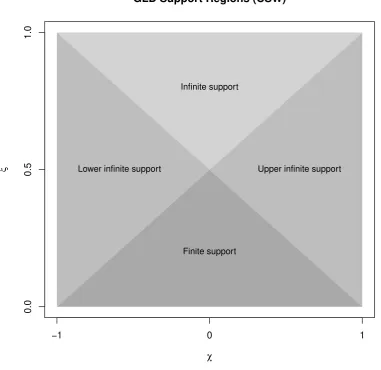
The GLD thus has unbounded infinite support, (_−∞,_∞), when ₂1(1_{− |}χ_|) _≤ξ; semi-infinite support bounded above, (_−∞, QCSW(1)], when χ < 0 and

1

2(1 +χ) ≤ ξ < 12(1−χ); and

semi-infinite support bounded below, [QCSW(0),∞), when 0< χand

1

2(1−χ)≤ξ < 12(1 +χ).

The distribution has finite support in the remaining region,ξ _≤ 1₂(1_{− |}χ_|).

As shown in Fig. 5, the support regions can be depicted using triangular regions in a shape plot with the asymmetry parameter χ versus steepness parameter ξ. This contrasts with the complex region supports of the RS parameterization displayed in Fig. 2. Of course, the region supports share the same intuitiveness as the FKML region supports in Fig. 3, since the shape-asymmetry parameterization is based on the FKML parameterization. The advantage of the CSW parameterization is that its shape parameters have finite domains of variation and the distribution family can therefore be represented by a single plot.

3.3 Moments

In this section, shape parameter (χ and ξ) dependent conditions for the existence of GLD moments are derived. As in Ramberg and Schmeiser [1974] and Freimer et al. [1988], conditions for the existence of moments can be determined by expanding the definition of thekth moment of the GLD into a binomial series where the binomial series can be represented by the Beta function. The existence condition of the moment then follow the existence condition of the obtained Beta function. In theλs representation of FKML in Eq. (2), the existence condition of thekth moment is min(λ3, λ4) >−1/k. For the parametersα and β defined in Eq. (7), this

gives the existence condition

min(α+β, α₋β)>₋1/k.

Some simple algebraic manipulation produces the condition of existence of thekth moment in terms of the shape parametersχ and ξ;

ξ < 1

2 −H |χ| −

r

4 4 +k2

! s

−1 0 1

0.0

0.5

1.0

GLD Support Regions (CSW)

χ

ξ

Infinite support

Lower infinite support Upper infinite support

Finite support

whereH is a discontinuous function such that

H(x) =

  

1 if x_≥0,

−1 otherwise,

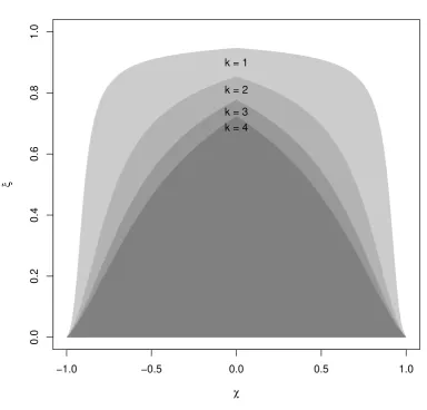
andβ is defined in Eq. (7b). Note that in the limiting cases of χ_{→ ±}1, the kth moment exists when and only when ξ_→0. Figure 6 shows the condition lines of existence for the first four moments in the shape diagram. Any set of shape parameters χ andξ that is under the kth condition line defines a distribution with a finitekth moment.

3.4 Tail behavior

The tail behavior plays an important role in the modeling of stochastic processes. This is especially the case for financial returns that have been shown to have fat tail distributions. An important class of distributions are the regularly varying tail distribution such as the Studentt, Fréchet,α-stable and Pareto distributions that exhibit power law decays. They are suitable for modeling the large and small values typically observed in financial data set. Moreover, power law distributions become very handy in the derivation of the asymptotic distribution of estimators such as the regression estimators encountered in econometric models [Jessen and Mikosch, 2006].

We now restrict our attention to the shape parameter range for which the GLD has infinite right tail,x_{→ ∞}; i.e., whenξ > 1₂(1₋χ) as shown in Eqs. (13) and (14). From Eq. (9),

x= ˜µ+ ˜σS(F(x)|χ, ξ)−S(

1 2|χ, ξ)

S(3_4|χ, ξ)₋S(1_4|χ, ξ) ,

whereS is defined in Eq. (8), α and β are defined in Eq. (7). In region ξ > 1₂(1₋χ),

lim

x→∞QCSW(x)∝(1−FCSW(x))

α−β

∝ β−_σ˜αx,

and hence

1₋FCSW(tx)

1₋F_CSW(x) ∼t

1/(α−β)_.

The right tail of the GLD is thus regularly varying at +_∞ with index _−α−1_β [see Embrechts et al., 1997, p. 129]. A similar argument shows that the left tail of the GLD is regularly varying at _−∞with index _−α+1_β.

−1.0 −0.5 0.0 0.5 1.0

0.0

0.2

0.4

0.6

0.8

1.0

GLD Moment Conditions

χ

ξ

k = 1

k = 2 k = 3 k = 4

the kth moments of the GLD is therefore infinite when k > max(_−α+1_β,_−α−1_β). This is in agreement with the existence conditions of moments presented in Section 3.3.

Moreover, from the monotone density theorem [Embrechts et al., 1997, Theorem A3.7], the density function is

f(x)_∝ 1

α₋β

β₋α

˜

σ x

1

α−β−1

asx_{→ ∞},

and with the analogous result asx_{→ −∞}. Hence, The decay exponent for the left and right tail of the probability density function are:

τ_left= 1

α+β −1, τ_right = 1

α₋β −1,

respectively. Since the left and right tail indices are related to the shape parametersχ andξ, the parameter estimates can be used to form an estimate of the tail indices.

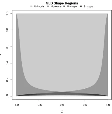
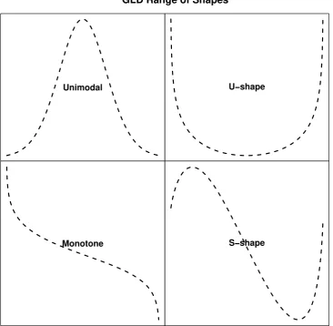
3.5 Distribution shape

The GLD exhibits four distribution shapes: unimodal, U-shape, monotone, and S-shape. In this section, conditions based on the derivatives of the quantile densityq in Eq. (11) are derived for each distribution shape. Indeed, the density quantile function is defined as the multiplicative inverse of the quantile density function, as noted in Eq. (10). The first and second derivatives ofq are

d

duq(u|σ, χ, ξ˜ )∝(α+β−1)u

α+β−2

−(α₋β₋1) (1₋u)α−β−2, (15a)

d2

du2q(u|σ, χ, ξ˜ )∝(α+β−1)(α+β−2)u

α+β−3₊

(α₋β₋1)(α₋β₋2) (1₋u)α−β−3, (15b) whereα andβ are defined in Eq. (7). It is now possible to deduce the parameter conditions for each of the four shape regions of the GLD. Figure 7 summarizes the shape regions as described in the remaining part of this section.

3.5.1 Unimodal

The GLD distribution is unimodal when its quantile density function is strictly convex; that is when _dud22q(u)>0for allu∈[0,1]. Note that throughout this paper, a unimodal distribution

refers to a distribution with a single local maximum. From Eq. (15b), the GLD density function is then unimodal when

−1.0 −0.5 0.0 0.5 1.0

0.0

0.2

0.4

0.6

0.8

1.0

GLD Shape Regions

χ

ξ

Unimodal Monotone U−shape S−shape

or when

α+β₋1<0 and α₋β₋1<0.

After some tedious but straightforward calculations, the conditions are, in terms of the shape parametersχand ξ,

0< ξ < 1

34

17₋4√17,

−2

r

4₋4α+α2

17₋16α+ 4α2 < χ <2 r

4₋4α+α2 17₋16α+ 4α2,

or

1 10

5₋2√5< ξ <1,

−2

r

1₋2α+α2

5₋8α+ 4α2 < χ <2 r

1₋2α+α2 5₋8α+ 4α2.

Figure 8 illustrates the unimodal distribution shapes of the GLD.

3.5.2 U-shape

Likewise, the GLD is U-shaped when the quantile density function is strictly concave, _dud22q(u)<0

for allu_∈[0,1]. This is the case when

0< α+β₋1<1 and 0< α₋β₋1<1,

giving the equivalent conditions

1 20

10₋3√10_≤ξ < 1

10

5₋2√5,

−2

r

1₋2α+α2

5₋8α+ 4α2 < χ <2 r

1₋2α+α2 5₋8α+ 4α2,

or

1 34

17₋4√17< ξ < 1

20

10₋3√10,

−2

r

4₋4α+α2

17₋16α+ 4α2 < χ <2 r

4₋4α+α2 17₋16α+ 4α2.

Figure 8 illustrates U-shaped distribution shapes of the GLD.

3.5.3 Monotone

The probability density function is monotone when its derivative is either positive or negative for all possible values in its support range. From Eq. (15a), this is the case when

χ =−0.768, ξ =0.004

χ =0, ξ =0.004

χ =0.768, ξ =0.004

χ =−0.514, ξ =0.337

χ =0, ξ =0.337

χ =0.514, ξ =0.337

χ =−0.301, ξ =0.034

χ =0, ξ =0.034

χ =0.301, ξ =0.034

χ =−0.218, ξ =0.018

χ =0, ξ =0.018

χ =0.218, ξ =0.018

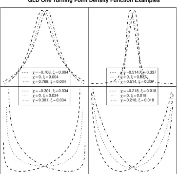
GLD One Turning Point Density Function Examples

or

α+β₋1<0 and α₋β₋1>0.

In terms of the shape parameters, the monotone shape conditions are

0< χ_≤ √2

5, 1

2−

s

1 + 2β+β2

5 + 8β+ 4β2 < ξ < 1 2−

s

1₋2β+β2 5₋8β+ 4β2,

or

2

√

5 < χ <1, 1

2−

s

1 + 2β+β2

5 + 8β+ 4β2 < ξ < 1 2+

s

1₋2β+β2 5₋8β+ 4β2,

or

−1< χ_{≤ −√}2

5, 1

2−

s

1₋2β+β2

5₋8β+ 4β2 < ξ < 1 2+

s

1 + 2β+β2 5 + 8β+ 4β2,

or

−√2

5 < χ <0, 1

2−

s

1₋2β+β2

5₋8β+ 4β2 < ξ < 1 2−

s

1 + 2β+β2 5 + 8β+ 4β2.

Figure 9 illustrates monotones shape of the GLD with different sets of shape parameters.

3.5.4 S-shape

Sinceα_∈Rand β_∈R, the remaining shape parameter regions are:

α+β >2 and 1< α₋β <2,

and

1< α+β <2 and α₋β >2.

χ =0.358, ξ =0.053

χ =0.537, ξ =0.058

χ =0.716, ξ =0.075

χ =0.947, ξ =0.428

χ =−0.947, ξ =0.082 χ =−0.537, ξ =0.058

χ =−0.358, ξ =0.053

χ =−0.179, ξ =0.052

GLD Monotone Density Function Examples

the gradient of the quantile density function has not the same sign for all possible values of the distribution. The GLD therefore has an S-shape density when

0< χ_≤ √1

2, 1

2 −

s

4 + 4β+β2

17 + 16β+ 4β2 < ξ < 1 2−

s

4₋4β+β2 17₋16β+ 4β2,

or

1

√

2 < χ <1, 1

2 −

s

4 + 4β+β2

17 + 16β+ 4β2 < ξ < 1 2 −

s

1 + 2β+β2 5 + 8β+ 4β2,

and

−1< χ_{≤ −√}1

2, 1

2 −

s

4₋4β+β2

17₋16β+ 4β2 < ξ < 1 2 −

s

1₋2β+β2 5₋8β+ 4β2,

or

−√1

2 < χ <0, 1

2 −

s

4₋4β+β2

17₋16β+ 4β2 < ξ < 1 2−

s

4 + 4β+β2 17 + 16β+ 4β2.

Figure 10 illustrates S-shaped probability densities of the GLD.

Sturges breaks The approach of Sturges [1926] is currently the default method for calculating

the number of histogram bins in theR _{Environment for Statistical Computing [R Core Team].}

Since Sturges’ formula computes bin sizes from the range of the data, it can perform quite poorly when the sample size is small in particular when,n is less than 30. For this method

bn=log2(n+ 1)

.

The brackets represent the ceiling function, by which log₂(n+ 1)will be rounded up to the next integer value.

Scott breaks Scott’s choice [see Scott, 1979] is derived from the normal distribution and relies

upon an estimate of the standard error. It offers a more flexible approach than the fixed number of bins used by Sturges. In Scott’s method, the number of bins is

bn=

l_{max(x)−min(x)}

h

m

χ =0.283, ξ =0.015

χ =0.424, ξ =0.015

χ =0.566, ξ =0.015

χ =0.824, ξ =0.013

χ =0.883, ξ =0.011

χ =0.941, ξ =0.007

χ =−0.883, ξ =0.011

χ =−0.824, ξ =0.013

χ =−0.766, ξ =0.015

χ =−0.424, ξ =0.015

χ =−0.283, ξ =0.015

χ =−0.141, ξ =0.015

GLD S−Shaped Density Function Examples

where

h= 3.49ˆσn1/3.

When all data are equal,h= 0, and bn= 1.

Freedman–Diaconis breaks The Freedman–Diaconis choice [Freedman and Diaconis, 1981] is

a robust selection method based upon the full and interquartile ranges of the data. The number of bins is

bn=

l_{max(x)−min(x)}

h

m

,

where

h= π(0.75)−π(0.25)

n1/3 .

If the interquartile range is zero, thenhis instead set to the median absolute deviation. The Sturges breaks do not use any information concerning the form of the underlying distri-bution, and so the Sturges histogram bins are often far from being optimal. The Scott approach is reliant upon the distribution being approximately normal, and so, for GLD applications, the histogram bins are not expected to be optimally chosen over the tails. Since it is a robust method based on the interquartile range, the Freedman–Diaconis approach seems to be the most promising option for creating histograms from random variates drawn from the heavy-tailed GLD.

3.6 Special cases

As seen in the previous section, the GLD can assume a wide range of distribution shapes. Here, values of the parameters in Eq. (9) are found such thatQ_CSW replicates several common distributions. The method used to accomplish this is as follows. Taking a set of equidistant probabilities, pi = _Ni₊₁, with i = 1, . . . , N and N = 500, the respective quantiles, xi, and

densities,di =f(xi), are calculated for each of the target distributions. The shape parameters, ˆ

χand ξˆ, are then fitted, by minimizing the maximum absolute quantile error (MQE):

sup

∀i |

QCSW(pi|µ,˜ σ,˜ χ,ˆ ξˆ)−xi|.

The median and interquartile range of the target distributions are used for the location and scale parameters,µ˜ andσ˜. Note thatN = 500was explicitly chosen in order to compare the results of this work with those of the previous studies of Gilchrist [2000], King and MacGillivray [2007] and Tarsitano [2010].

Distribution Parameters χˆ ξˆ sup|Qˆ| sup|Fˆ| sup|fˆ|

Normal µ= 0, σ= 1 0.0000 0.3661 0.012 0.001 0.001

Student’st ν= 1 0.0000 0.9434 1.587 0.005 0.012

ν= 5 0.0000 0.5778 0.069 0.003 0.004

ν= 10 0.0000 0.4678 0.033 0.002 0.003

Laplace µ= 0, b= 1 0.0000 0.6476 0.257 0.015 0.093

Stable α= 1.9, β= 0 0.0000 0.5107 0.399 0.010 0.010

α= 1.9, β= 0.5 0.0730 0.5307 0.584 0.014 0.013

Gamma k= 4, θ= 1 0.4120 0.3000 0.120 0.008 0.012

χ2 k= 3 0.6671 0.1991 0.295 0.015 0.072

k= 5 0.5193 0.2644 0.269 0.011 0.017

k= 10 0.3641 0.3150 0.233 0.007 0.004

Weibull k= 3, λ= 1 0.0908 0.3035 0.007 0.003 0.016

Log Normal µ= 0, σ= 0.25(log scale) 0.2844 0.3583 0.011 0.007 0.052

Gumbel α= 0.5, β= 2 -0.3813 0.3624 0.222 0.010 0.010

Inv. Gaussian µ= 1, λ= 3 0.5687 0.2957 0.096 0.022 0.175

µ= 0.5, λ= 6 0.3267 0.3425 0.008 0.008 0.125

NIG µ= 0, δ= 1, α= 2, β= 1 0.2610 0.4975 0.124 0.014 0.029 Hyperbolic µ= 0, δ= 1, α= 2, β= 1 0.2993 0.4398 0.198 0.021 0.030

Table 2: Shape parameters of the GLD to approximate common distributions.

error,sup_|Fˆ_|, and the maximum density error,sup_|fˆ_|. The maximum probability error (MPE) is defined as

sup

∀i |

FCSW(xi|µ,˜ σ,˜ χ,ˆ ξˆ)−pi|.

The maximum density error (MDE) is defined as

sup

∀i |

f_CSW(xi|µ,˜ σ,˜ χ,ˆ ξˆ)−di|.

−5 0 5

0.0

0.1

0.2

0.3

0.4

Exact Location and Scale

MQE = 0.307 x

f(x)

−5 0 5

Fitted Location and Scale

MQE = 0.097 x

Figure 11: Approximation of the Studentt-distribution (dotted lines) with two degrees of freedom by either fitting or using the true values for the location and scale parameters, µ˜ and

˜

σ. In the left-hand-side figure, the fitted GLD where the true values for the median and interquartile range were used. In the right-hand-side figure, the location and scale parameters were included in the estimation. Note the maximum quantile error (MQE) for the left hand side figure, 0.307_{, is larger than the one for the right hand}

side figure,0.097_{, although it has a better visual fit.}

is not well described by the latter solution. Using the known values forµ˜andσ˜ yields a greater MQE value (of 0.307_{, in this case) than that of the alternate approach (for which, the MQE}

value was 0.097_).

−15 −5 0 5 10 15

0.002

0.010

0.050

0.200

1.000

Minimum MQE

MPE = 0.005 x

F(x)

−15 −10 −5 0 5 10 15

Minimum MPE

MPE = 0.001 x

Figure 12: Comparison of the fitted GLD (dotted lines) to the Studentt-distribution with two degrees of freedom by either using the MQE or the MPE estimator. The left-hand-side figure was obtained by minimizing the MQE and the right-hand-left-hand-side plot with the MPE. The MPE for the left hand side plot, 0.005_{, is larger than the one for the}

˜

µ σ˜ χ ξ

Uniform(a, b) 1

2(a+b)

1

2(b−a) 0

1

2 −

1

√

5 1

2(a+b)

1

2(b−a) 0

1

2−

2

√

17

Logistic(µ, β) µ βln(9) 0 1₂

Exponential(λ) 1

λln(2)

1

λln(3) 1 0

Table 3: Special cases of the GLD in the CSW parameterization.

Another important consideration in our approach is to ensure that the fitted parameters yield a GLD with a support that includes all xi. This is especially the case for the gamma,χ2 and

Wald distributions. Indeed, it is possible to find parameter-value sets for which the MQE is small, but where the fitted distribution does not include allxi. We therefore add constraints in

the optimization routine to ensure that allxi are included in the fitted GLD support range.

These considerations motivated the decisions to use the known values for the location and scale parameters, to ensure that all points are included in the support of the fitted distribution, and to use the MQE estimator to fit the shape parameters.

The GLD includes the uniform, logistic, and exponential distributions as special cases. The corresponding GLD parameter values, obtained from Eqs. (8), (9) and (12), are summarized in Table 3. Note that the exponential distribution corresponds to the limiting case_{χ_→1, ξ_→0_}, as mentioned at the end of Section 3.1.

4 Parameter estimation

Estimating parameter values for the generalized lambda distribution (GLD) is notoriously difficult. This is due to abrupt distribution shape changes that accompany variations of the parameter values in the different shape regions (Fig. 2). In this section, an extensive Monte-Carlo study of different GLD estimators is presented. This includes maximum log-likelihood, maximum product of spacing, goodness-of-fit, histogram binning, quantile sequence, and linear moments. Besides these estimators, we introduce the maximum product of spacing and a robust moment matching to estimate the shape parameters of the GLD.

4.1 Robust moments matching

The method suggested by Ramberg et al. [1979] for fitting GLD distributions, uses a method of moments wherein the first four moments are matched. Clearly, this approach can only be applied to regions within the first four moments exist. In addition, parameter estimates based upon sample moments are highly sensitive to outliers. This is especially true of third and fourth moment. To circumvent the estimation of sample moments, Karian and Dudewicz [1999] considered a quantile approach that estimates the parameters from four sample quantile statistics. In that approach, the four statistics depend upon the four parameters of the GLD, thereby leading to a system of four nonlinear equations to be solved.

In the CSW parameterization, because the location and scale parameters are, respectively, the median and interquartile range, they can be directly estimated by their sample estimators. What remains to be estimated, are two shape parameters; χand ξ. This is achieved by using the robust skewness ratios˜of Bowley [1920], and the robust kurtosis ratio˜κ of Moors [1988]. These robust moments are defined as

˜

s= π3/4+π1/4−2π2/4

π_3/4−π_1/4 ,

˜

κ= π7/8−π5/8+π3/8−π1/8

π_6/8−π_2/8 ,

where πq indicates theqth quantile, and the tilde indicates the robust versions of the moments.

For a detailed discussion of Bowley’s skewness and Moors’ kurtosis statistics, please refer to [Kim and White, 2004].

Recall that the quantile function of the GLD in the CSW parameterization is

QCSW(u|µ,˜ σ, χ, ξ˜ ) = ˜µ+ ˜σ

S(u_|χ, ξ)₋S(1_2|χ, ξ)

S(3_4|χ, ξ)₋S(1_4|χ, ξ),

as seen in Eq. (9) whereS is defined in Eq. (8). The population robust skewness and robust kurtosis thus depend only upon the shape parameters. Explicitly,

˜

s= S(3/4|χ, ξ) +S(1/4|χ, ξ)−2S(2/4|χ, ξ)

S(3/4_|χ, ξ)₋S(1/4_|χ, ξ) , (16a) ˜

κ= S(7/8|χ, ξ)−S(5/8|χ, ξ) +S(3/8|χ, ξ)−S(1/8|χ, ξ)

S(6/8_|χ, ξ)₋S(2/8_|χ, ξ) . (16b)

4.2 Histogram approach

The histogram approach is appealing and simple; the empirical data are binned in a histogram and the resulting probabilities, taken to be at the midpoints of the histogram bins, are fitted to the true GLD density. This approach was considered by Su [2005] for the GLD. To obtain the best estimates, it is vital to choose an appropriate number of bins for the histogram. Three different methods of estimating the number of bins were investigated. In the following discussions of these,n denotes the sample size, andbn denotes the number of bins for that sample size.

4.3 Goodness-of-fit approaches

To test the goodness-of-fit of a continuous cumulative distribution function, to a set of data, statistics based on the empirical distribution function can be used. Examples of these are the Kolmogorov–Smirnov, Cramér–von Mises, and Anderson–Darling statistics. These statistics are measures of the difference between the hypothetical GLD distribution and the empirical distribution.

To use these statistics as parameter estimators, they are minimized with respect to the unknown parameters of the distribution. It is known, from the generalized Pareto distribution, that these approaches are able to successfully estimate the parameters even when the maximum likelihood method fails. This is shown by Luceño [2006], who calls this approach the method of maximum goodness-of-fit. Definitions and computational forms of the three goodness-of-fit statistics named above are also given in the paper of Luceño [2006].

The following discussions consider a random sample ofn iid observations,_{x1, x2, . . . , xn},

with the order statistics of the sample denoted by_{x₍₁₎, x₍₂₎, . . . , x_(n)}, and writeFi =F(x(i))

the corresponding probability of the eventx(1).

4.3.1 The Kolmogorov–Smirnov statistic

The Kolmogorov–Smirnov statistic measures the maximum distance between the empirical cumulative distribution function and the theoretical probabilities, Sn;

Dn= sup

x |Fx−Sn(x)|,

where the sample estimator is

c

Dn= 1

2n+ max1≤i≤n

Fi−

1₋i/2

n

.

4.3.2 The Cramér–von Mises statistic

The Cramér–von Mises statistic uses mean-squared differences, thereby leading to a continuous objective function for parameter optimization:

W_n2 =n

Z ∞

∞

[Fx−Sn(x)]2dF(x),

which reduces to

d

W2

n =

1 12n+

n

X

i=1

Fi−1−i/2

n

2

.

4.3.3 The Anderson–Darling statistic

The Anderson–Darling statistic is a tail-weighted statistic. It gives more weight to the tails and less weight to the center of the distribution.

This makes the Anderson–Darling statistic an interesting candidate for estimating parameters of the heavy-tailed GLD. It is defined as

A2_n=n

Z ∞

∞

[Fx−Sn(x)]2

F(x)(1₋F(x))dF(x),

where its sample estimator is

c

A2

n=−n− 1

n

n

X

i=1

(2i₋1)(ln(Fi) + ln(1₋Fn+1−i).

4.4 Quantile matching

As described by Su [2010], the quantile matching method consists of finding the parameter values that minimize the difference between the theoretical and sample quantiles. This approach is especially interesting for the GLD, since the distribution is defined by a quantile function.

Consider an indexed set of probabilities, p, as a sequence of values in the range0< pi<1.

The quantile matching estimator is defined For a cumulative probability distribution F with a set of parametersθ, the quantile matching estimator yield the parameter values

ˆ

θ= arg min θ 1 n n X i

(F−1(pi|θ)−Q(pi))2,

where nis the cardinality of p,F−1_{(p|θ) is the quantile function, and Qthe sample quantile}

function.

4.5 Trimmed L-moments

combinations of the ordered data values. The method of L-moments is to find the distribution parameter values that minimize the difference between the sample L-moments and the theoretical ones. Elamir and Seheult [2003] introduced the trimmed L-moments, a robust extension of the L-moments.

The trimmed L-moments, lr(t1, t2), on the order statisticsX1:n, . . . , Xn:n of a random sample

X of sizenwith trimming parameters t1 and t2, are defined as

T L(r, t1, t2) = 1

r

r−1 X

k=0 (₋1)k

r₋1

k

E[r+t1−k, r+t1+t2], (17)

where

E[i, r] = r! (i₋1)!(r₋i)!

Z 1

0

Q(u)ui−1(1₋u)r−i.

Qis the quantile function of the distribution. Note that when t1=t2 = 0, this reduces to the

definition of the standard L-moment. The concept behind the trimmed L-moments is to extend the sample size byt1+t2 and trim the t1 smallest andt2 largest order statistics.

Using the unbiased estimator of the expectation of the order statistics,E, of Downton [1966], Elamir and Seheult [2003] obtains the sample estimatorEˆ:

ˆ

E(i, r) = 1_n r n X t=1

t₋1

i₋1

n₋t r₋i

Xt:n,

which can be used to estimate the sample’srth trimmed L-moment in Eq. (17).

The derivation of the trimmed L-moments for the GLD is cumbersome. Asquith [2007] calculated them for the RS parameterization.

4.6 MLE and MPS approaches

The Kullback–Leibler (KL) divergence [Kullback, 1959], also known by the names informa-tion divergence, informainforma-tion gain, and relative entropy, measures the difference between two probability distributions: P and Q. Typically,P represents the empirical distribution, andQ

comes from a theoretical model. The KL divergence allows for the interpretation of many other measures in information theory. Two of them are the maximum log-likelihood estimator and the maximum product of spacing estimator.

4.6.1 Maximum log-likelihood estimation

The maximum log-likelihood method was introduced by Fisher [1922]. For a more recent review, please refer to Aldrich [1997]. Consider a random sample ofniid observations, _{x1, x2, . . . , xn}

drawn from the probability distribution with parameter setθ. Then the maximum value of the log-likelihood function,_L, defined by

L(θ) = n

X

returns optimal estimates for the parameters θ of the probability density function f. The maximum of this expression can be found numerically using a non-linear optimizer that allows for linear constraints.

4.6.2 Maximum product of spacing estimation

The maximum likelihood method may break down in certain circumstances. An example of this is when the support depends upon the parameters to be estimated [see Cheng and Amin, 1983]. Under such circumstances, the maximum product of spacing estimation (MPS), introduced separately by Cheng and Amin [1983]; Ranneby [1984], may be more successful. This method is derived from the probability integral transform, wherein the random variates of any continuous distribution can be transformed to variables of a uniform distribution. The parameter estimates are the values that make the spacings between the cumulative distribution functions of the random variates equal. This condition is equivalent to maximizing the geometric means of the probability spacings.

Consider the order statistics,_{x₍₁₎, x₍₂₎, . . . , x_(n)}, of the observations _{x1, x2, . . . , xn}, and

compute their spacings or gaps at adjacent points,

Di =F x(i)

−F x_(i−1)

,

where F x₍₀₎ = 0 and F x_(n+1) = 1. The estimate of the maximum product of spacing becomes

ˆ

θ= arg max θ∈Θ

n+1 X

i=1

lnD(x_(i)).

The maximizing solution can be found numerically with a non-linear optimizer.

Note that the concept underlying the MPS method is similar to that of the starship estimation GLD estimation method introduced by King and MacGillivray [1999]. However, the starship method uses the Anderson–Darling test to find the parameters that make the spacings closest to a uniform distribution.

4.7 Empirical study

In this section, we compare the aforementioned estimators. In this study we specifically take: the Anderson–Darling statistic for the goodness-of-fit approach, the Friedman–Diaconis breaks for the histogram approach, the L-moments estimator, the MLE, the MPS estimator, the quantile matching estimator, the robust moment matching and the trimmed L-moments estimator with

t1= 1 andt2 = 1. All methods have been implemented for the GLD in the statistical software

Figure 13 shows the fitted log-density of the GLD for the Google equity log-returns with the different methods. Overall, The estimates differ by small amounts in the lower tail. However, the upper tail fit of the histogram approach is substantially different from the other methods.

To compare the estimation methods, we generated one thousand time series of one thousand points each, for each of the set GLD parameter sets: _{µ˜ = 0,σ˜ = 1, χ = 0, ξ = 0.35_}. We perform both approaches, when the location and scale parameters,(χ, ξ), are estimated by their sample estimators, and when they are included in the estimator. Table 4 shows the median and interquartile range of the minimum discrimination information criterion (MDE). The MDE is a divergence between two distributions measure used in information statistics. The MDE between two continuous distributions,f andg, is defined as

Dφ(f, g) =

Z ∞

−∞ φ

f(x)

g(x)

g(x)dx,

where

φ(x) =₋log(x)₋x+ 1.

A divergence measure is used to evaluate how closely the estimator can fit the distribution. This is in contrast to the traditional mean absolute deviation and mean absolute error of the parameter estimates, which focus on how closely the estimator can fit the parameters. The distinction is important because, although the fitted parameters might substantially differ from those used to generate the time series, their combination can produce a fitted distribution that closely resembles the generating distribution. Table 4 also shows how many of the estimation routines have successfully converged to a minimum, and the median computation times. From the results, the performance of the estimators in terms of the MDE is not affected by estimating the parameter values of the GLD using the two-step procedure: the location and scale parameter estimated by their sample estimates, and the two shape parameter values fitted by the estimator into consideration. However, the computation times of convergence are much shorter in the former case. This is expected, since the optimization routine only seeks solutions for the shape parameters, leading to a simpler optimization path. This result can be useful when dealing with a large data set, in which case the computation time is commonly critical.

5 Applications

5.1 Shape plot representation

● ● ● ● ● ● ●●● ● ●● ●● ● ● ● ● ● ● ● ● ● ● ●●● ● ● ● ● ● ● ● ● ● ●●●● ● ● ● ● ● ● ● ● ● ● ● ● ● ●●● ● ● ●● ● ● ●● ● ● ● ● ● ● ● ● ● ● ●● ● ● ● ● ●● ● ● ● ● ● ●

−10 −5 0 5 10 15 20

−8 −6 −4 −2 x log f(x) ad hist lm mle mps quant shape tlm

GOOG Parameter Estimation

sample(˜µ,σ˜) optim(˜µ,σ˜)

MDE conv. time [s] MDE conv. time [s]

mle 0.0022 (2.50E-03) 100% 0.15 0.0019 (1.94E-03) 100% 0.43 hist 0.0046 (5.29E-03) 100% 0.01 0.0054 (5.85E-03) 100% 0.02 prob 0.0069 (7.49E-03) 100% 0.14 0.0048 (5.55E-03) 100% 0.34 quant 0.0030 (3.74E-03) 100% 0.02 0.0021 (2.50E-03) 100% 0.03 shape 0.0090 (1.44E-02) 100% 0.01 0.0090 (1.44E-02) 100% 0.01 ad 0.0035 (3.84E-03) 100% 0.14 0.0026 (2.50E-03) 100% 0.36 mps 0.0022 (2.21E-03) 100% 0.10 0.0018 (1.76E-03) 100% 0.19

(a) With no outliers

sample(˜µ,σ˜) optim(˜µ,σ˜)

MDE conv. time [s] MDE conv. time [s]

mle 0.0082 (6.64E-03) 100% 0.16 0.0073 (5.70E-03) 100% 0.37 hist 0.0070 (1.10E-02) 100% 0.01 0.0071 (6.40E-03) 100% 0.02 prob 0.0069 (7.14E-03) 100% 0.14 0.0051 (5.27E-03) 100% 0.35 quant 0.0047 (4.77E-03) 100% 0.01 0.0045 (5.18E-03) 100% 0.03 shape 0.0086 (1.33E-02) 100% 0.01 0.0086 (1.33E-02) 100% 0.01

ad 0.0055 (4.88E-03) 96% 0.20 0.0042 (3.20E-03) 91% 0.40

mps 0.0101 (7.25E-03) 100% 0.09 0.0088 (6.34E-03) 100% 0.19

(b) With 1% of outliers with scale d = 3

sample(˜µ,σ˜) optim(˜µ,σ˜)

MDE conv. time [s] MDE conv. time [s]

mle 0.1391 (1.41E-02) 100% 0.14 0.1300 (1.38E-02) 100% 0.48 hist 0.1968 (8.52E-03) 100% 0.01 0.8170 (2.27E-01) 100% 0.04 prob 0.0585 (1.99E-02) 100% 0.14 0.0578 (1.92E-02) 100% 0.40 quant 0.1259 (8.93E-03) 100% 0.02 0.2061 (5.00E-02) 100% 0.03 shape 0.0400 (2.36E-02) 100% 0.01 0.0400 (2.36E-02) 100% 0.01 ad 0.1174 (1.78E-02) 100% 0.12 0.1155 (1.77E-02) 100% 0.34 mps 0.1418 (1.39E-02) 100% 0.12 0.1329 (1.36E-02) 100% 0.23

(c) With 10% of outliers with scale d = 10

AKAM CHRW DLTR FISV KLAC MSFT ORCL RIMM SYMC XLNX

AMAT CMCSA EBAY FLEX LIFE MU ORLY ROST TEVA XRAY

CA COST ERTS FLIR LLTC MXIM PAYX SBUX URBN YHOO

CELG CSCO ESRX HSIC LRCX MYL PCAR SIAL VOD

CEPH CTSH EXPD INFY MAT NTAP PCLN SNDK VRSN

CERN CTXS FAST INTC MCHP NVDA QCOM SPLS VRTX

CHKP DELL FFIV INTU MICC NWSA QGEN SRCL WFMI

Table 5: NASDAQ Symbols. The 66 components of the NASDAQ-100 index that have records from 2001–01–03 to 2011–12–31.

the tails. The shape plot is thus ideal for comparing the fitted shape parameters of a data set between different time series. This section illustrates the use of the shape plot with shape parameters fitted to equities from the NASDAQ-100 index.

The NASDAQ-100 index comprises 100 of the largest US domestic and international non-financial companies listed on the NASDAQ stock market. The index reflects the share prices of companies across major industry groups, including computer hardware and software, telecommu-nications, retail and wholesale trade, and biotechnology. The listed equity returns are expected to exhibit a wide range of distribution shapes. The GLD is therefore a good candidate for modeling their various distributions. The NASDAQ-100 financial index series financial index series used in this study has records from 2000–01–03 to 2011–12–311_{. These are listed in}

Table 5. The log-returns of the adjusted closing prices were used. Note that the survivor bias [Elton et al., 1996] has not been considered in this experiment, because the objective is merely to illustrate the use of the GLD with real time series data.

First, the location and scale parameters were estimated from their sample estimators. The maximum likelihood estimator is then used to fit the shape parameters,χ andξ. Figure 15 shows the fitted shape parameters. It is interesting to note that the fitted parameters are to the symmetric vertical line at χ= 0. However, the fitted shape parameters have values that are well above those that best describe the standard normal distribution; these are represented by a triangle in the shape plot. The GLDs fitted to the NASDAQ data have “fatter” tails than does the normal distribution. This is one of the so-called stylized facts of financial returns.

This example is important because it illustrates how the GLD can model time series with tails that are fatter than those of the normal distribution. The ability of the GLD to model time series with different types of tails could be used in an assets selection process. For example, assets could be classified according to their kurtosis order, which is along the vertical access of the GLD shape plot.

1_{Data downloaded from}

−1.0 −0.5 0.0 0.5 1.0

0.0

0.2

0.4

0.6

0.8

1.0

GLD Shape Plot

χ

ξ

Figure 14: This figure illustrates the different probability density shapes for various steepness and asymmetry parameters. The location and scale of the distribution are, respectively,

˜

−1.0 −0.5 0.0 0.5 1.0 0.0 0.2 0.4 0.6 0.8 1.0

GLD Shape Plot

NASDAQ−100 χ ξ ● ● ● ● ● ● ● ● ● ● ●_● ● ● ● ● ● ● ● ● ● ● ● ● ● ● ● ● ● ● ● ● ● ● ● ● ● ● ● ● ● ● ● ● ● ● ● ● ● ● ● ● ● ● ● ● ● ● ● ● ● ● ● ● ● ●

5.2 Quantile based risk measures

Two risk measures commonly used in portfolio optimization are the value-at-risk (VaR) and the expected shortfall risk (ES). On one hand, the VaRγ is the maximum loss forecast that may

happen with probabilityγ _∈[0,1]given a holding period. On the other hand, the ESγ is the

averaged VaRγ in the confidence interval [0, γ]. These risk measures are thus related to the

quantiles of the observed equity price sample distribution. Since the quantile function takes a simple algebraic form, these two risk measures are easily calculated:

VaRγ=QCSW(γ|µ,˜ σ, χ, ξ˜ ), and

ESα = 1

γ

Z γ

0

VaRνdν = 1

γ

Z γ

0

Q_CSW(ν_|µ,˜ σ, χ, ξ˜ )dν

=                           

γ(B+ ˜µ+Alnγ) + (A₋Aγ) ln(1₋γ) if χ= 0, ξ= 1₂,

γµ˜+Aγ(₂1_α+ lnγ₋1) +A(1−₂γ_α)₊₄1+2_αα2−1+Bγ if χ6= 0, ξ= 1₂(1 +χ),

Aγ(−1+4β2_+γ2β₎

2β(1+2β) +γ(B+ ˜µ) + (A−Aγ) ln(1−γ) if χ6= 0, ξ= 12(1−χ),

A (1₋γ)1+α₋(1₋γ)β(1₋γ)−β (α₋β)(1 +α₋β) +Bγ

+ Aγ

α₋β − Aγ α+β +

Aγ1+α+β

(α+β)(1 +α+β) +γµ˜ otherwise,

whereQ_CSW is defined in Eq. (9),α and β are defined in Eq. (7), and

A= ˜σ[S(3/4_|χ, ξ)₋S(1/4_|χ, ξ)]−1, B =₋[S(3/4_|χ, ξ)₋S(1/4_|χ, ξ)]−1.

5.3 Apparent scaling law

This section follows the examples of Barndorff-Nielsen and Prause [2001], wherein the normal inverse Gaussian distribution (NIG) has been used to demonstrate the existence of an apparent scaling law for financial returns. By repeating that exercise with the GLD, the ability of the GLD to model both financial returns and the NIG will be demonstrated.

[1995] observed the same scaling law in the US dollar and Deutschmark (USD/DEM) exchange rates. Herein, the volatility is defined as the average of absolute logarithm price changes. The volatility over a duration time, τ, is

vτ =h|xt−xt−τ|i

where xt= ln_PP_tt

−1

are the logarithm returns andPt are the prices at timet. There is a scaling

law

vτ =

_τ

T

H

vT,

where T is an arbitrary time interval andH is the scaling law index factor. In the last decade, several new scaling laws have been reported. The interested reader may wish to refer to [Glattfelder et al., 2011] for a review of known scaling laws.

Barndorff-Nielsen and Prause [2001] have shown that the apparent scaling of the volatility of high-frequency data is largely due to the semi-heavy-tailedness of financial distributions. The scaling parameter,H, can be estimated by a linear regression on the logarithm of the scaling relation in the scaling law.

Figure 16 displays the scaling laws of random variates generated by the GLD with location parameterµ˜ = 0, scale parameterσ˜= 5_×10−4_{, and shape parameter χ= 1. It is clear that}

varying the skewness parameterξ of the GLD changes the scaling constant (i.e., the regression coefficient in the log-log transform). This is a good illustration of how a semi-heavy fat-tailed distribution can reproduce a scaling law, and of how the GLD parameters can be modified to obtain a desired scaling constant.

Another typical effect of the temporal aggregation of financial data is the Gaussianization of the aggregated financial returns. For high-frequency data, the returns are usually modeled by fat-tailed distributions, since the normal distribution has the wrong shape. However, when the returns are aggregated over long time intervals, the empirical distribution of the aggregated returns is observed to converge onto the normal distribution. Figure 17 illustrates this effect with the USD/DEM exchange rate. The data set consists of the hourly returns of USD/DEM from January 1, 1996 at 11 p.m. to December 31, 1996 at 11 p.m. Figure 17 shows the fitted GLD shape parameters of the 1, 6, 12, 24, and 60 hour aggregated logarithm returns. The fitted shape parameters appear to be converging onto the normal distribution located at approximately

(χ= 0, ξ = 0.366)as reported in Table 2.

In Fig. 18, the same experiment has been performed with US dollar and Swiss Franc (USD/CHF) exchange rate tick data for the years 2004, 2006, 2008 and 20102_{. The aggregated}

returns can be seen to converge in distribution to a normal distribution.

2_{The exchange rate tick data was provided by}

● ● ● ● ● ● ● ● ● ● ● ● −8.0 −7.0 −6.0

Scaling Power Law of GLD

log(n)

log(E|X_n|)

regression coefficient: 0.529 GLD skewness: ξ =0.4

● ● ● ● ● ● ● ● ● ● ● ● −8.0 −7.0 −6.0

Scaling Power Law of GLD

log(n)

log(E|X_n|)

regression coefficient: 0.548 GLD skewness: ξ =0.7

● ● ● ● ● ● ● ● ● ● ● ● −7.5 −6.5 −5.5

Scaling Power Law of GLD

log(n)

log(E|X_n|)

regression coefficient: 0.608 GLD skewness: ξ =0.85

● ● ● ● ● ● ● ● ● ● ● ● −7.0 −6.0 −5.0 −4.0

Scaling Power Law of GLD

log(n)

log(E|X_n|)

regression coefficient: 0.694 GLD skewness: ξ =0.9

Figure 16: Scaling power law of random variates generated by the GLD with location parameter

˜

µ= 0, scale parameterσ˜ = 5_×10−4_{, and shape parameterχ= 1. The remaining}

−1.0 −0.5 0.0 0.5 1.0

0.0

0.2

0.4

0.6

0.8

1.0

GLD Shape Plot

χ

ξ

1 6

12

24

60

−0.4 −0.2 0.0 0.2 0.4

0.2

0.4

0.6

0.8

GLD Shape Plot (2004)

χ

ξ

1 h 6 h 9 h

12 h 24 h

−0.4 −0.2 0.0 0.2 0.4

0.2

0.4

0.6

0.8

GLD Shape Plot (2006)

χ

ξ

1 h

6 h 9 h 12 h 24 h

−0.4 −0.2 0.0 0.2 0.4

0.2

0.4

0.6

0.8

GLD Shape Plot (2008)

χ

ξ

1 h 6 h 9 h 12 h 24 h

−0.4 −0.2 0.0 0.2 0.4

0.2

0.4

0.6

0.8

GLD Shape Plot (2010)

χ

ξ

1 h 6 h 9 h

12 h 24 h

6 Conclusion

This paper has introduced a new parameterization of the GLD, which provides an intuitive interpretation of its parameters. The median and interquartile range are respectively synonymous with the location and scale parameters of the distribution. The shape parameters describe the asymmetry and steepness of the distribution. This parameterization differs from previous parameterizations, where the asymmetry and steepness of the GLD is expressed in terms of both tail indicesλ3 and λ4 of Eqs. (1) and (2). Another advantage of this new parameterization, is

that the location and scale parameters can be equated to their sample estimators. This reduces the complexity of the estimator used to fit the remaining two shape parameters. However, this new parameterization comes with the cost of having more intricate expressions for both the conditions of existence for the moments, and the conditions on the shape parameters for the different distribution shapes. Nevertheless, evaluating these expressions remains straightforward. Moreover, the new parameterization enables the use of shape plots that can be used to represent the fitted parameters. Furthermore, value-at-risk, expected shortfall, and the tail indices can be expressed by simple formulae, dependent upon the parameters.

The GLD with unbounded support is an interesting, power-law tailed, alternative to the

α-stable and the Student t-distribution for purposes of modeling financial returns. The key advantage of the GLD is it can accommodate a large range of distribution shapes. A single distribution can therefore be used to model the data for many different asset classes; e.g., bonds, equities, and alternative instruments. This differs from current practice where different distributions must be employed, corresponding to the different distributional shapes of the data sets. Another point, which is often overlooked in practice, is that the same distribution can be applied to different subsets of the data. For example, the distribution of the returns might completely change from year to year. The GLD would then be able to capture this distributional change.

Due to its flexibility, the GLD is a good candidate for studying structural changes of a data set by Bayesian change-point analysis. This may be of use in the identification of market-change regimes.

The R packagegldistimplements the new GLD parameterization, along with the parameter estimation methods that have been presented in this work.

Acknowledgments