Index Terms —: Extended Backward Differentiation

(1)



Abstract— An application of three steps Extended Block Backward Differentiation Formulae (EBBDF) for the

solutions of semi-explicit index-1 systems of Differential Algebraic Equations (DAEs) is presented. The processes compute the solutions of DAEs in a block by block fashion by some continuous schemes which are combined and implemented as a set of block formulae. Numerical results revealed this method to be efficient and very accurate, and particularly suitable for semi implicit index one DAEs.

Index Terms—: Extended Backward Differentiation

Formula, Block method, L-Stability I. INTRODUCTION

A system of ordinary differential equations(ODEs) with algebraic constraints which can be written in form





 



(

),

(

),

(

)

(



)

₀

,

 

(

1

)

'

0 0 2

0 0 1







z

x

z

x

z

x

y

f

y

x

z

x

y

x

y

is called differential algebraic equation.

DEFINITION 1.1 (Differential index): The index along the solution path is defined as the minimum number of differentiations of the system (1) that is required to reduce the system to a set of ODEs .

Numerical solutions for DAEs were first introduced by Gear by applying numerical methods for ODEs to DAEs [4]. Runge-Kutta methods [1] and BDF [2], [5] are commonly used for semi-explicit index-1 DAEs, however, these methods approximate the solution of (1) at one point. The algorithm presented in this paper is based on block method and approximates the solution at several points. It

Manuscript received January 22, 2013; revised February 22, 2013.. O. A.. Akinfenwa is with the department of Mathematics, University of Lagos, Nigeria (corresponding author phone: +2347057175195; e-mail: [email protected]).

S. A. Okunuga is with the department of Mathematics, University of Lagos, Nigeria (e-mail: [email protected]).

would be observed that block methods were first introduced by Milne [9] for use only as a means of obtaining starting values for predictor-corrector algorithms and has since then been developed by several researchers (see [4,10,11,12]), for general use. This paper presents a block method which preserves the Runge-Kutta traditional advantage of being self-starting and is more efficient than several known methods, since it requires m function evaluations per integration step, where m is the number functions in the block method .

II. DERIVATION OF THE METHOD

In this section, we develop an Extended Backward Differential equation (EBDF) with the additional methods derived from its first derivative and combined to form the Extended Block Backward Differentiation Formula (EBBDF) on the interval from

x

_nto

x

_n_₃



x

_n



3

h

where h is the chosen step-length. In particular, we assume that the exact solution y(x) on the interval



x

_n

,

x

_n_₃



is locally represented by Y (x) given by



 



1

0

)

(

)

(

s r

j

x

l

x

Y



(2)

where

l

_j are unknown coefficients to be determined, and

)

(

x

j



are polynomial basis function of degree

r



s



1

. such that the number of interpolation points

r

and the number of distinct collocation points,

s

are respectively chosen to satisfy

r



k

,

s



0

. The proposed method is thus constructed by specifying the following parameters:,



(

x

_n__j

)



x

_nj__j

,

j



0

,

1

,

.

.,

4

2

,

3



s

r

, and

k



3

.

by imposing the following conditions

2

,

1

,

0

,

4

0



_

 



l

x

y

_n _i

i

j j

i n

j (3)

,

3

,

2

,

4

0

1



 

 



jl

x

f

_n _i

i

j

j i n

j

(4)

assuming that ynj Y



xn ih



denote the numerical

approximation to the exact solution y

 

x_n_j ,

Solving Semi-Explicit Index-1 DAE Systems

using L-Stable Extended Block Backward

Differentiation Formula with Continuous

Coefficients

Olusheye.A. Akinfenwa and Solomon.A. Okunuga

(2)



x ih



Y

f_n_j   _n  denote the approximation to y

 

xnj ,

n

is the grid index. It should be noted that equations (3) and (4) lead to a system of five equations which is solved by matrix inversion to obtain the coefficients

l

_j j0,1,...,4. The EBDF with continuous coefficients is then obtained by substituting these values of

l

_j into equation (2). After some algebraic computation, the method yields the expression in the form

 

2

 



₂

 

₂ ₃

 

₃



 

5

0      





n j n n

j

j x y h x f x f

x

Y   

where



_j

(

x

)

, j=0, 1, 2, 2(x),3(x) are continuous

coefficients. The continuous coefficients of equation (5) are thus given as

.

  



₄

 

2



0 ₆₈ 5 5 17 2 h x x h x x h x x h

x _   n   n   n

 ,

  



 

₄2



1 ₁₇ 7 7 24 2 h x x h x x h x x

x _  n   n   n



,

  







4









2 2 2 68 143 23 228 h x x h x x h x x h x x

x _  n   n   n    n 

,

  



3







2 ₃₄ 11 39 2 h x x h x x h x x h x x

x _  n   n   n    n



,

 





₃





2 3 ₁₇ 2 h x x h x x h x x

x __  n   n   n



is then used to generate the main discrete EBBDF by evaluating at point

x



x

_n_₃to yield

 

6 17 6 17 18 y 17 9 y 17 9 y 17 1

- n 1 n 2 2 3

3    

  n   n  n

n f f

y

Differentiating (5) with respect to x we have

 

1 2

 



₂

 

₂ ₃

 

₃



,

 

7

0 

        _ _ _ 



n j n n

j j f x f x h y x h x

Y   

) (x

j



, j=0, 1, 2;

2(x)

,

3(x) are continuouscoefficients

used to generate the additional methods.

The additional methods are obtained by evaluating (7) at points x



xn, xn₁



to obtained

) 8 ( 17 4 17 39 y 17 57 y 17 96 y 17 39

-  n1 n2 2 3

 n n n

n f f

f

) 9 ( 17 1 17 14 y 17 27 y 17 24 y 17 3

- _n₁ _n ₂ ₂ ₃

1    

  n   n  n

n f f

f

the methods (6), (8), and (9), are combined to give the Extended block BDF 10

III. ORDER OF ACCURACYAND STABILTY OF EBBDF

The three step extended block backward differentiation formulae can be represented by a matrix finite difference equation in block form as

        ₍₁₁₎

1 0 1 1 0 1      _ _ _

 A Y hB F hB F

Y A

where

Y







y

_n1

,

y

_n2

y

_n3



T,

Y

__₁





y

_n_₂

,

y

_n_₁

y

_n



T,





T n n

n

f

F





1 2 3 ,





T n n

n f f

f

F1  2 1

.

,

2

,

1

,

0





and n0,3,...,N3.

And the matrices _A 1_,_A 0_,_B 1 are ₃_by₃ matrices whose entries are given by the coefficients of (11) given as

, 1 17 9 17 9 0 17 57 17 96 0 17 27 17 24 ) 1 (                      A , 17 1 0 0 17 39 0 0 17 3 0 0 ) 0 (                     A _, 17 6 17 18 0 17 4 17 39 0 17 1 17 14 1 ) 1 (                     B            0 0 0 1 0 0 0 0 0 ) 0 ( B

The local truncation error associated with the EBBDF can be defined to be the linear difference operator





(12)

] ; ) (

[ 2 2 3 3

2 0      





n n

j

j n

jy h f f

h x y

L   

Assuming that y(x) is sufficiently differentiable, we can write the terms in (12) as a Taylor series expression of

 

xn j

y  and f

 

xnj =y

 

xnj as



 )

(xn j

y



  

0 ) ( ! ) ( j n p _x y p jh

and

) (xn j y 

 



    0

1₍ ₎ ! ) ( j n p p x y p jh

(13) Substituting (13) into equation (12), we obtain the equation

] ; ) ( [y x h

L _n _{ } _{ } 2 _{ } . . . _{ } . . .

2 1

0       

 Cyx Chy x Chy x Chpypx p

Where the constants C_p , p0,1,2,. . .are given as follows:





2 0 0 J j

C



. . . 3 2 ! 2 1 3 2 2 1 2 2 l J j j

C 



     

              



(2 3 )

! 1 1 3 1 2 1 2 1 l p p p J j p

p _p j p l

C    

(3)

The method in (10) is said to have a maximal order of accuracy p if

1 1

 

2

1 ] ; ) (

[  _    p

n p p p

n h C h y x Oh x

y L

And

0 ,

0 . .

. 1

2 1

0  C C Cp  Cp 

C (14)

Therefore,

C

_p_₁is the error constant and p p _{ }_n p h y x

C 1 1

1

  

the principal local truncation error at the point

x

_n.

Therefore the values of the error constant calculated for the EBBDF (10) is given as:

T

   



 _ 

51 1 , 170

19 , 170

13

with order p=(4,4,4)

T

and

T is the transpose.

A. Zero Stability

The zero stability of the method is concerned with the stability of the difference system in the limit as h tends to zero [6]. Thus, as h0 the difference system (11) becomes

A

 

1Y  A

 

0Y1

whose first characteristics polynomial



 

R

given

by

R_j 1, j 1, ...,3

   





(1 )

17 72 det

)

(_R _ _RA1 __A0 _ _R2 __R



. (15)

The block method (10) is zero stable for 

 

R =0 and satisfies, and for those roots with

R

_j



1

, the multiplicity does not exceed 1. hence the extended block BDF with continuous coefficients is zero stable.

B. Consistency and Convergence

We note that the block method (10) is consistent as it has order

p



1

. Since the block method (10) is zero stable then following Henrici [8],

Convergence = zero stability + consistency, hence the method (10) converges.

C. Linear Stability

The stability properties of the block formulae (10) is discussed and determined through the application to the test equation :

y







y

,





0

(16) applying (12) on (16) yields

Y





Q

(

z

)

Y





1

, (17) where

Q

(

z

)

is the amplification matrix with

z



h



given by

Q

(

z

)

=

(

A

(1)



zB

 1

)

1

.(

A

(0)



B

(0)

)

The matrix

Q

(

z

)

has eigenvalues





₁

,



₂

,



₃

 



0

,

0

,



₃



,

where the dominant eigenvalue



₃ is a rational function of

z

given by

 

3 2

3

z 3 -z 11 z 18 -12

z 3 z 11 z 18 12



 

  z

 (18)

which is the stability function of our block method (10). From (18) the usual property of A-stability which requires that for all

z



h





C

 and



3

(

z

)



0

is obtained. The

absolute stability region

S

associated with the block method (10) is the set



z h

S  .for that z where the roots of the stability function (18)



1 moduli

are .

In the spirit of Hairer and Wanner [7], the stability region

S

is presented in white colour which corresponds to the 3- step extended block BDF stability function (18). Clearly, from Figure 1 below, it is obvious that the method is A- stable, since it has no pole of the stability function (18) represented by the plus sign in the left half complex plane, also (18) satisfies the L- stability condition that

Re

(

)



0





z

im

L

z where

z



h



.

Therefore, the method is L-Stable.

Figure1.Absolute stability region

IV.

Computing with EBBDF

The method is implemented more efficiently as a 3-step block numerical integrators for (1) to simultaneously obtain the approximations



y

_n_₁

,

y

_n_₂

,

y

_n_₃



T without requiring back values or predictors taking n  0,3,..., N 3 over sub-intervals



x0, x3



,...,



x_N3,x_N



. For example, n =

0,



= 1,



y

₁

,

y

₂

,

y

₃



T are simultaneously obtained over the sub-interval



x

₀

,

x

₃



, as

y

₀ is known from the initial value problem (1), n=3,



=2, .





T

y y

y₄, ₅, ₆ are simultaneously obtained over the sub-interval



x₃,x₆



as

S

Unstable

(4)

3

y

is known from previous block and so on. Hence, the sub-intervals do not over-lap. It should be noted that for linear problems, the code used Gaussian elimination and for nonlinear problems, the Newton’s method is used.

V. NUMERICAL EXAMPLEs

In this section, we give three examples to illustrate the accuracy of the method. The three problems are standard DAE problems whose solutions are of importance in applied systems. We find maximum absolute errors of the approximate solution. All computations were carried out using our written Mathematica code in Mathematica 8.0.

Example 5.1

0 ) 0 ( ,

0 sin

1 ) 0 ( , ) 1 ( cos

) (

 



 

  



z z

x

y z x y

x x x y

,,,,,,,,,,,

The exact solution is

x

z

x

e

x

y

(

)



x



sin

,

(

)



sin

Example 5.2

1 ) 0 ( ,

0 , (0) 1

) (

2

3 _  _ _



z y

zy x z y 10

0  x

3 2

3 1 ) ( , 3 1 )

( 

       

     

 x z x x

x y

Example 5.3

0 ) 0 ( ,

2 sin 5

1 ) 0 ( ,

2 cos 5

1 ) 0 ( , ) 1 ( )

(

5 ) 0 ( , ) 1 ( )

(

2 2

1 2

2 1

2 2 1

2

1 1 2

1

 

      

  

      

 

   

 

   

z x

z y

z x

z y

y z x xy

x y

y z x xy

x y

10 0  x

x x

z x x

z

x x

x y

x x

x y

sin ) ( , cos ) (

, 2 sin 5 cos ) (

, 2 cos 5 sin ) (

2 1

2 2

2 1

 



       

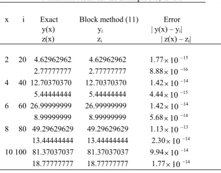
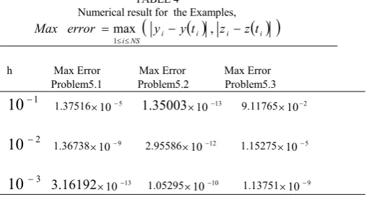
[image:4.595.313.537.72.232.2]

The tables below show the numerical results of extended block BDF method for solving semi-explicit index-1 DAEs. Tables 1, 2, 3 display the result for example 5.1, 5.2, and 5.3 for h=0.1, while for different step size the maximum errors are obtained in table 4.

TABLE 1

Numerical result for the Example 5.1, h=0.1

x i Exact Block method (11) Error y(x) yi | y(x) – yi|

z(x) zi

| z(x) – zi|

2 20 1.95393014 1.95393606 5.92_₁₀6

0.90929743 0.90929861 1.18_₁₀6

4 40 –3.00889434 –3.00889931 4.97_₁₀6

–0.75680249 –0.75680352 1.03_₁₀6

6 60 –1.67401423 –1.67402028 6.04_₁₀6

–0.27941549 –0.27941584 3.50_₁₀7

8 80 7.91520143 7.91521420 1.27_₁₀5

0.98935824 0.98935949 1.25_₁₀6

10 100 –5.44016570 –5.44017306 7.36_₁₀6

[image:4.595.314.539.284.460.2]

–0.54402111 –0.54402190 7.90_₁₀7

TABLE 2

x i Exact Block method (11) Error y(x) yi | y(x) – yi|

z(x) zi

| z(x) – zi|

2 20 4.62962962 4.62962962 1.77_₁₀15

2.77777777 2.77777777 8.88_₁₀16

4 40 12.70370370 12.70370370 1.42_₁₀14

5.44444444 5.44444444 4.44_₁₀15

6 60 26.99999999 26.99999999 1.42_₁₀14

8.99999999 8.99999999 5.68_₁₀14

8 80 49.29629629 49.29629629 1.13_₁₀13

13.44444444 13.44444444 2.30_₁₀14

10 100 81.37037037 81.37037037 9.94_₁₀14

18.77777777 18.77777777 1.77_₁₀14

TABLE 3

x Exact Exact Method (11) Method (11) Error Error y(x1) y(x2) y1 y2 | y(x1)-y1| | y(x2)–y2|

z(x1) z(x2) z1 z2

| z(x1)–z1| | z(x2)-z2|

2 -1.171437 0.416147 -1.171279 0.416035 1.58_₁₀4 _1.12_₁₀4

4.130340 0.909297 4.130540 0.909322 2.00_₁₀4₂_.49_₁₀5

4 -1.484303 0.653644 -1.484763 0.652627 4.60_₁₀4₁_.02_₁₀3

4.293148 -0.756802 4.295901 -0.756771 2.75_₁₀3₃_.16_₁₀5

6 3.022168 -0.960170 3.031045 -0.954886 8.88_₁₀3₅_.28_₁₀3

-2.794766 -0.279415 -2.807775 -0.275101 1.30_₁₀2₄_.31_₁₀3

8 5.160475 0.145500 5.181067 0.136285 2.06_₁₀2₉_.21_₁₀3

2.611633 0.989358 2.612052 0.992150 4.19_₁₀4_2.79_₁₀3

(5)

[image:5.595.56.320.56.200.2]

TABLE 4

Numerical result for the Examples,

 



i i i i



NS

i y y t z z t

error

Max   



 ,

max

1

h Max Error Max Error Max Error

Problem5.1 Problem5.2 Problem5.3

1

10

 _1.37516_₁₀5_1.35003_₁₀13_9.11765_₁₀2

2

10

 _1.36738_₁₀9_2.95586_₁₀12_1.15275_₁₀5

3

10

 3.16192_₁₀13_1.05295_₁₀10_1.13751_₁₀9

VI CONCLUSION

We have proposed in this paper a EBBDF for the solutions of semi-explicit index-1 DAEs. The method is of order 4, it is self-starting and provides good accuracy. Numerical examples using the three step EBBDF showed that the method is accurate and efficient as evident in Tables 1-3. The EBBDF is also found to be convergent and L-stable, making it a suitable , method this class of problems.

REFERENCES

[1] U.M. Ascher and L.R. Petzold, Projected Implicit Runge-Kutta Methods for Differential Algebraic Equations, SIAM J. Numer. Anal., 28, 1991, pp. 1097–1120.

[2] K. E. Brennan, S.L. Campbell and L. R. Petzold, Numerical Solution of Initial Value Problems in Di erential-Algebraic Equations, Elsevier, New York, 1989.

[3] L. G. Brita and O.A. Rabia, Parallel Block Predictor-Corrector Methods for ODEs, IEEE transactions on Computers, C-36(3), 1987, 299–311.

[4] C. W. Gear, Simultaneous Numerical Solution of Di erential-Algebraic Equations, IEEE Trans. Circuit Theory, CT-18, 1971, pp.89–95.

[5] C.W. Gear and L.R. Petzold, ODE System for the Solution of Differential Algebraic Systems, SIAM J. Numer. Anal., 28, 1984, pp.1097–1120.

[6] S.O. Fatunla, Block methods for second order IVPs, Intern. J. Comput. Math. 41, 1991, pp. 55–63.

[7] E. Hairer, G. Wanner, Solving Ordinary Differential Equations II, Springer, New York, 1996.

[8] P. Henrici, Discrete Variable Methods in ODEs, John Wiley, New York, 1962.

[9] W. E. Milne, Numerical solution of differential equations, John Wiley and Sons, 1953.

[10] J. D. Rosser, A Runge-Kutta for all seasons, SIAM, Rev., 9, 1967, pp. 417-452.

[11] D. Sarafyan Multistep methods for the numerical solution of ordinary differential equations made self-starting, Tech. Report 495, Math. Res. Center, Madison 1965.