ISSN 2307-7743 http://scienceasia.asia
_______________
Key words and phrases: Block method, Ninth stage, Runge-Kutta type method, Uniform order and Computational stable.
© 2016 Science Asia 1 / 12
DERIVATION OF NINTH STAGE RUNGE-KUTTA METHOD FOR THE SOLUTION OF FIRST ORDER DIFFERENTIAL EQUATIONS
MSHELIA DW, BADMUS AM AND YAKUBU DG
Abstract: We present hybrid block of eight integrators which are of uniform order nine through interpolation and collocation procedures. The properties of the hybrid block integrators are fully investigated and confirmed to be computationally stable also the block method derived are reconstructed to ninth stage Runge-Kutta method which implemented on stiff, physical and life problems. The results obtained compare favourably with the existing methods when implemented in Runge-Kutta mode.
1.0 Introduction
Among the most important mathematical tools used in producing models in the physical sciences, Biological sciences and Engineering are differential equations. But most of these differential equations do not posses closed form or finite solutions. Even if they posses closed form solutions we do not know the method of getting them.
In many real-life situations, the differential equation that models the problem is too complicated to solve exactly. Hence there is need to develop an accurate algorithm for obtaining an equivalent approximating solution to the original problems. Most recent researchers have developed some block methods to cater for this class of problems
𝑦′= 𝑓(𝑥, 𝑦), 𝑦(𝑎) = 𝜌 (1)
Among such researchers are [1], [2],[3], [4] , [5],[6] and [7] to mention a few.
In our method, a block of eight integrators were proposed at step length of four which are of uniform order nine and also all the discrete schemes in our block came from a single continuous formula
Definition 1.0 Zero stable
A linear multi-step method is said to be Zero-stable if the roots 𝑅𝑗, 𝑗 = 1(1)𝑘 of the first characteristics polynomials
𝜌(𝑅) = 𝑑𝑒𝑡 [∑ 𝐴𝑖𝑅𝑘−𝑖
𝑘
𝑖=0
] = 0, 𝐴0 = −1, 𝑠𝑎𝑡𝑖𝑠𝑓𝑖𝑒𝑠 |𝑅𝑗| ≤ 1
2.0 Development of the method
Our objective is to derive a block of eight integrators of the form
𝑦(𝑥𝑛+𝑣) =∝0 𝑦𝑛 + ℎ [𝛽0𝑓𝑛 + 𝛽3 4
𝑓
𝑛+34+ 𝛽1𝑓𝑛+1+ 𝛽32𝑓𝑛+32+ 𝛽2𝑓𝑛+2+ 𝛽52𝑓𝑛+52+ 𝛽3𝑓𝑛+3
+ 𝛽7 2
𝑓
𝑛+72+ 𝛽4𝑓𝑛+4] (2)
where 𝑥𝑛+𝑣 , 𝑣 = 3
4 ,1, 3 2 ,2,
5 2 ,3,
7 2 , 4.
We proceed by seeking an approximate solution of the form
𝑦(𝑥) = ∑ ∝𝑗 𝑚+𝑡−1
𝑗=0
𝑥𝑗 (3)
𝑦′(𝑥) = ∑ 𝑗 ∝ 𝑗 𝑚+𝑡−1
𝑗=1
𝑥𝑗−1=𝑓(𝑥, 𝑦) (4)
where 𝑚 and 𝑡 are the number of collocation and interpolation points used in the method. Specifically for this method 𝑚 = 9 , 𝑡 = 1 and the degree of the polynomial is 𝑚 + 𝑡 − 1. Equation (3) is interpolated at 𝑥 = 𝑥𝑛 and (4) is collocated at
𝑥 = 𝑥𝑛+𝑣, 𝑣 = 0, 3 4 , 1,
3 2, 2,
5 2, 3,
7 2 3
and 4 which leads to the following non linear system of equations of the form
𝑃(𝑥) = ∑ ∝𝑗 𝑚+𝑡−1
𝑗=0
𝑥n𝑗
𝑃′(𝑥) = ∑ 𝑗 ∝ 𝑗 𝑚+𝑡−1
𝑗=1
𝑥𝑛+𝑣𝑗−1 = ℎ ∑ 𝛽𝑗
𝑚+𝑡−1
𝑗=0
(x)𝑓𝑛+𝑣 = 𝑓(𝑥, 𝑦) (5)
When using Maple 17 (Mathematical software) to determine the unknown parameters ∝𝑗
and 𝛽𝑗 in (5), we obtain the following.
∝0= 𝑦𝑛
𝛽0 = [𝑙 −18027 7560ℎ𝑙
2+ 71277
22680ℎ2𝑙
3− 2732
1080ℎ3𝑙
4+ 6989
5400ℎ4𝑙
5 − 1369
3240ℎ5𝑙
6+ 161
1890ℎ6𝑙 7
− 73
7560ℎ7𝑙8+
4
8505ℎ8𝑙9]
𝛽3 4
= [4096(2520) 405405ℎ 𝑙
2−8192(8658)
1216215ℎ2 𝑙3+
2048(1745) 57915ℎ3 𝑙4−
8192(1316) 289575ℎ4 𝑙5+
4096(575) 173745ℎ5 𝑙6
−16384(73) 405405ℎ6 𝑙7+
4096(35) 405405ℎ6𝑙8−
65536 3648645ℎ8𝑙9]
𝛽1 = [−7560 180ℎ𝑙
2 +28494
270ℎ2𝑙3−
42783 360ℎ3𝑙4+
33713 450ℎ4𝑙5−
7605 270ℎ5𝑙6+
2(989) 315ℎ6 𝑙7−
69 90ℎ6𝑙8
+ 16
𝛽3 2
= [2(252) 135ℎ 𝑙
2−4(10338)
405ℎ2 𝑙3+
1(16867) 135ℎ3 𝑙4−
4(1425) 675ℎ4 𝑙5+
2(6805) 405ℎ5 𝑙6−
16(463) 945ℎ6 𝑙7
+2(67) 135ℎ6𝑙8−
64 1215ℎ8𝑙9]
𝛽2 = [−1(1890)
60ℎ 𝑙
2 +1(16137)
180ℎ2 𝑙
3−1(13785)
120ℎ3 𝑙
4+1(24463)
300ℎ4 𝑙
5−1(6115)
180ℎ5 𝑙
6+1(867)
105ℎ6 𝑙 7
−1(65) 60ℎ6 𝑙8+
8 135ℎ8𝑙9]
𝛽5 2
= [4(1512) 315ℎ 𝑙
2−8(6606)
945ℎ2 𝑙3+
2(1659) 45ℎ3 𝑙4−
8(1522) 225ℎ4 𝑙5+
4(789) 135ℎ5 𝑙6−
32(58) 315ℎ6 𝑙7+
4(63) 315ℎ6𝑙8
− 128
2835ℎ8𝑙 9]
𝛽3 = [−
1(2520) 324ℎ 𝑙
2 +1(11178)
486ℎ2 𝑙3−
1(20033) 648ℎ3 𝑙4+
1(18821) 810ℎ4 𝑙5−
1(5017) 486ℎ5 𝑙6+
2(761) 567ℎ6 𝑙7
−1(61) 162ℎ6𝑙8+
16 729ℎ8𝑙9]
𝛽7 2
= [2(1080) 1155ℎ 𝑙
2−4(4842)
3465ℎ2 𝑙3+
1(1257) 165ℎ3 𝑙4−
4(1202) 825ℎ4 𝑙5+
2(655) 495ℎ5 𝑙6−
16(51) 1155ℎ6𝑙7+
2(59) 1155ℎ6𝑙8
− 64
10395ℎ8𝑙9]
𝛽4 = [−1(4215) 14040ℎ 𝑙
2+ 1(8541)
14040ℎ2𝑙3−
1(3921) 4680ℎ3 𝑙4+
1(15203) 23400ℎ4 𝑙5−
1(4215) 14040ℎ5𝑙6+
1(671) 8190ℎ6𝑙7
− 1(57) 4680ℎ6𝑙
8+ 4
5265ℎ8𝑙
9]
(6) where 𝑙 = (𝑥 − 𝑥𝑛)
𝑦(𝑥) =∝0 𝑦𝑛+ ℎ [𝛽0𝑓𝑛+ 𝛽3 4
𝑓
𝑛+34+ 𝛽1𝑓𝑛+1+ 𝛽32𝑓𝑛+32+ 𝛽2𝑓𝑛+2+ 𝛽52𝑓𝑛+52+ 𝛽3𝑓𝑛+3
+ 𝛽7 2
𝑓𝑛+7 2
+ 𝛽4𝑓𝑛+4] (7)
Equation (6) is substituted in equation (7) to obtain our continuous formula. Also evaluating (7) at 𝑥 = 𝑥𝑛+𝑣, 𝑣 =
3 4 ,1,
3 2 ,2,
5 2 ,3 ,
7
2 𝑎𝑛𝑑 4 to yield eight integrators to form
our hybrid block methods as follows:
[
1 0 0 0 0 0 0 0 0 1 0 0 0 0 0 0 0 0 1 0 0 0 0 0 0 0 0 1 0 0 0 0 0 0 0 0 1 0 0 0 0 0 0 0 0 1 0 0 0 0 0 0 0 0 1 0 0 0 0 0 0 0 0 1]
[ 𝑦𝑛+3
4
𝑦𝑛+1 𝑦
𝑛+32
𝑦𝑛+2
𝑦
𝑛+52
𝑦𝑛+3
𝑦
𝑛+72
𝑦𝑛+4] =
[
0 0 0 0 0 0 0 1
0 0 0 0 0 0 0 1
0 0 0 0 0 0 0 1
0 0 0 0 0 0 0 1
0 0 0 0 0 0 0 1
0 0 0 0 0 0 0 1
0 0 0 0 0 0 0 1
0 0 0 0 0 0 0 1]
[ 𝑦𝑛−13
4
𝑦𝑛−3 𝑦
𝑛−52
𝑦𝑛−2 𝑦
𝑛−32
𝑦𝑛−1
𝑦
𝑛−12
+ℎ
[
985667
400400 −
72842607 22937600
14005219
5734400 −
89105481 45875200
72842607
22937600 −
2085791 4587520 46741504
18243225 −
340769 113400
102397
42525 −
72607
37800
16082 141750 −
91943 204120 4848
1925 −
244719 89600
61343
22400 −
360477
179200 1881 1600 −
8327 17920 46235648
18243225 −
39386 14175
128144
42525 − 8098
4725 2272
2025 −
11462 368550 1841200
729729 −
797975 290304
641525
217728 −
271175
193536 50135
36288 −
1247875 2612736 63488
25025 − 3897
1400 527
175 − 2133
1400 306
175 − 71 280 502544
200475 −
2809513 1036800
2243563
777600 −
916153 691200
194089 129600
368039 1866240 48234496
18243225 −
43072
14175
145408 42525 −
9896
4725 32768
14175 −
11584 25515
6797493 63078400 −
1372587 1192755200 973
7425 −
8413 737100 27081
246400 −
4203 358400 5552
51975 −
4213 368550 29675
266112 −
178775 15095808 27
275 − 99 9100 272629
950400 −
64141 4147200 47104
51975
24242 184275 ]
[ 𝑓
𝑛+34 𝑓𝑛+1 𝑓
𝑛+32 𝑓𝑛+2 𝑓
𝑛+52 𝑓𝑛+3 𝑓
𝑛+72 𝑓𝑛+4]
+ ℎ
[
0 0 0 0 0 0 0 16196113 91750400 0 0 0 0 0 0 0 59977 340200 0 0 0 0 0 0 0 63341
358400 0 0 0 0 0 0 0 15011
85050 0 0 0 0 0 0 0 615535
3483648 0 0 0 0 0 0 0 247
1400 0 0 0 0 0 0 0 2202641 12441600 0 0 0 0 0 0 0 1058
6075 ] [
𝑓 𝑛−134 𝑓𝑛−3 𝑓
𝑛−5 2 𝑓𝑛−2 𝑓
𝑛−32 𝑓𝑛−1 𝑓
𝑛−12 𝑓𝑛 ]
(8)
Let 𝐴(0) =
[
1 0 0 0 0 0 0 0
0 1 0 0 0 0 0 0
0 0 1 0 0 0 0 0
0 0 0 1 0 0 0 0
0 0 0 0 1 0 0 0
0 0 0 0 0 1 0 0
0 0 0 0 0 0 1 0
By multiplying (8) by the inverse of 𝐴(0) and rearrange it in Butcher Table as
𝐶 𝐴
3 16 16196113 91750400 985667 400400 − 72842607 22937600 14005219 5734400 − 89105481 45875200 72842607 22937600 − 2085791 4587520 6797493 63078400 − 1372587 1192755200 1 4 59977 340200 46741504 18243225 − 340769 113400 102397 42525 − 72607 37800 16082 141750 − 91943 204120 973 7425 − 8413 737100 3 8 63341 358400 4848 1925 − 244719 89600 61343 22400 − 360477 179200 1881 1600 − 8327 17920 27081 246400 − 4203 358400 1 2 15011 85050 46235648 18243225 − 39386 14175 128144 42525 − 𝟖𝟎𝟖𝟗 4725 2272 2025 − 11462 𝟐𝟓𝟓𝟏𝟓 5552 51975 − 4213 368550 5 8 615535 3483648 1841200 729729 − 797975 290304 641525 217728 − 271175 193536 50135 36288 − 1247875 2612736 29675 266112 − 178775 15095808 3 4 247 1400 63488 25025 − 3897 1400 527 175 − 2133 1400 306 175 − 71 280 27 275 − 99 9100 7 8 2202641 12441600 502544 200475 − 2809513 1036800 2243563 777600 − 916153 691200 194089 129600 368039 1866240 272629 950400 − 64141 4147200
1 1058 6075 48234496 18243225 − 43072 14175 145408 42525 − 9896 4725 32768 14175 − 11584 25515 47104 51975 24242 184275 1 1058
6075 48234496 18243225 − 43072 14175 145408 42525 − 9896 4725 32768 14175 − 11584 25515 47104 51975 24242 184275 (9) The Table (9) satisfies Runge-Kutta conditions for solution of first order ODEs since
(𝒊) ∑ 𝒂𝒊𝒋= 𝒄𝒊 𝒔
𝒋=𝟏
(𝒊𝒊) ∑ 𝒃𝒋 = 𝟏 𝒔
𝒋=𝟏
The method (8) is formally given as Runge-Kutta type method as
9 8 7 6 5 4 3 2 1 1 368550 12121 51975 11776 25515 2896 14175 8192 4725 2474 42525 36352 14175 10768 18243225 12058624 12150 529 k k k k k k k k k h y
yn n
k1 f
xn,yn
9 8 7 6 5 4 3 2 1 2 4771020800 13732587 252313600 6797493 18350080 2085791 11468800 3285531 183500800 89105481 22937600 14005219 91750400 7284260 1601600 985667 367001600 16196113 , 16 3 k k k k k k k k k h y h x f
9 8 7 6 5 4 3 2 1 3 2948400 8413 29700 793 816480 91943 28350 8041 151200 72607 170100 102397 453600 340769 18243225 11685376 1360800 59977 , 4 1 k k k k k k k k k h y h x f
k n n
9 8 7 6 5 4 3 2 1 4 1433600 4203 985600 27081 71600 8327 6400 1881 716800 360477 89600 61343 358400 244719 1925 1212 1433600 63341 , 8 3 k k k k k k k k k h y h x f
k n n
9 8 7 6 5 4 3 2 1 5 1474200 4213 51975 1388 51030 5731 2025 568 9450 4049 42525 32036 28350 19693 18243225 11558912 340200 15011 , 2 1 k k k k k k k k k h y h x f
k n n
9 8 7 6 5 4 3 2 1 6 60383232 178775 1064448 29675 10450944 1247875 145152 50135 774144 271175 870912 641525 1161216 797975 729729 460300 13934592 615535 , 8 5 k k k k k k k k k h y h x f
k n n
9 8 7 6 5 4 3 2 1 7 36400 99 1100 27 1120 71 350 153 5600 2133 700 527 5600 3897 25025 15872 5600 247 , 4 3 k k k k k k k k k h y h x f
k n n
9 8 7 6 5 4 3 2 1 8 16588800 64141 3801600 272629 7464960 368039 518400 194089 2764800 916153 3110400 2243563 4147200 2809513 200475 125636 49766400 2202641 , 8 7 k k k k k k k k k h y h x f
k n n
9 8 7 6 5 4 3 2 1 9 368550 12121 51975 11776 25515 2896 14175 8192 4725 2474 42525 36352 14175 10768 18243225 12058624 12150 529 , k k k k k k k k k h y h x f
k n n
(10) 3.0 Consistency and Stability of the block method
Thus obtain the normalized form of (8),the first characteristics polynomial of the normalized matrix will be expressed as
𝜌(𝑧) =
| | |
𝜆
(
1 0 0 0 0 0 0 0 0 1 0 0 0 0 0 0 0 0 1 0 0 0 0 0 0 0 0 1 0 0 0 0 0 0 0 0 1 0 0 0 0 0 0 0 0 1 0 0 0 0 0 0 0 0 1 0 0 0 0 0 0 0 0 1)
−
(
0 0 0 0 0 0 0 1
0 0 0 0 0 0 0 1
0 0 0 0 0 0 0 1
0 0 0 0 0 0 0 1
0 0 0 0 0 0 0 1
0 0 0 0 0 0 0 1
0 0 0 0 0 0 0 1
0 0 0 0 0 0 0 1)
| | |
= 𝟎
𝜆7(𝜆 − 1) = 0
𝜆1 = 0, 𝜆2 = 0, 𝜆3 = 0, 𝜆4 = 4, 𝜆5 = 0, 𝜆6 = 0, 𝜆7 = 0, 𝜆8 = 1
From definition 1.0, the newly hybrid block method (8) is zero stable and also consistent since the order of all the integrators are uniform order 9 > 1
4.0 Numerical Experiments
The following examples are used to confirm the efficiency of our method Example 4.1
𝑦′= 20𝑥2− 20𝑦 + 2𝑥, 𝑦(0) =1
3 ℎ = 0.05 0 ≤ 𝑥 ≤ 1.0 Exact Solution: 𝑦(𝑥) = 𝑥2+1
3𝑒 −20𝑥
Example 4.2
𝑦′= −𝑦, 𝑦(0) = 1 ℎ = 0.05 0 ≤ 𝑥 ≤ 1.0 Exact Solution: 𝑦(𝑥) = 𝑒−𝑥
Example 4.3 (SIR Model)
The Susceptible Infected Recovery (SIR) model is an epidemiological model that computes the theoretical number of people infected with a contagious illness in a closed population over time. The name of this class of models derives from the fact that they involve coupled equations relating the number of susceptible people 𝑆(𝑡), number of people infected 𝐼(𝑡), and the number of people who have recovered 𝑅(𝑡),. This is a good and simple model for many infectious diseases including measles, mumps and rubella. It is given by the following three coupled equations.
𝑑𝑆
𝑑𝑡 = 𝜇(𝐼 − 𝑆) − 𝛽𝐼𝑆 𝑑𝐼
𝑑𝑡= 𝜇𝐼 − 𝛾𝐼 + 𝛽𝐼𝑆 (i) 𝑑𝑅
𝑑𝑡 = 𝜇𝑅 + 𝛾𝐼
where 𝜇, 𝛾 and 𝛽 are positive parameters. Define 𝑦 to be,
𝑦 = 𝑆 + 𝐼 + 𝑅 (𝑖𝑖) when solutions in (i) are substituted in (ii) we have
𝑦′ = 𝜇(1 − 𝑦)𝑡 then
Taking 𝜇 = 0.5 and attaching an initial condition 𝑦(0) = 0.5 (for a particular closed population), we obtain
𝑦′= 0.5(1 − 𝑦), 𝑦(0) = 0.5 (𝑖𝑣) Exact solution: 𝑦(𝑡) = 1 − 0.5𝑒−0.5𝑡
Example 4.4
𝑦′= 𝜆(𝑠𝑖𝑛𝑥 − 𝑦), 𝑦(0) = 0 ℎ = 0.05 0 ≤ 𝑥 ≤ 1.0
Exact Solution: 𝑦(𝑥) = 𝜆2
𝜆2+1𝑠𝑖𝑛𝑥 − 𝜆
𝜆2+1𝑐𝑜𝑠𝑥 + 𝜆 𝜆2+1𝑒
−𝜆𝑥
Absolute errors, with stiffness ratio 𝜆 = 100 for fixed step size ℎ = 0.01, 0 ≤ 𝑥 ≤ 1.0
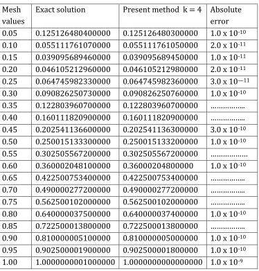
Table 1: Approximate solution of Example 4.1 at k=4
Mesh values
Exact solution Present method k = 4 Absolute error 0.05 0.125126480400000 0.125126480300000 1.0 x 10⁻¹⁰
0.10 0.055111761070000 0.055111761050000 2.0 x 10⁻¹¹
0.15 0.039095689460000 0.039095689450000 1.0 x 10⁻¹¹
0.20 0.046105212960000 0.046105212980000 2.0 x 10⁻¹¹
0.25 0.064745982330000 0.064745982360000 3.0 x 10—11
0.30 0.090826250730000 0.090826250760000 1.0 x 10⁻¹⁰
0.35 0.122803960700000 0.122803960700000 ……….. 0.40 0.160111820900000 0.160111820900000 ……….. 0.45 0.202541136600000 0.202541136300000 3.0 x 10⁻¹⁰
0.50 0.250015133300000 0.250015133200000 1.0 x 10⁻¹⁰
0.55 0.302505567200000 0.302505567200000 ……… 0.60 0.360002048100000 0.36000204800000 1.0 x 10⁻¹⁰
0.65 0.422500753400000 0.422500753400000 ……….. 0.70 0.490000277200000 0.490000277200000 ……….. 0.75 0.562500102000000 0.562500102000000 ……….. 0.80 0.640000037500000 0.640000037400000 1.0 x 10⁻¹⁰
0.85 0.722500013800000 0.722500013800000 ……….. 0.90 0.810000005100000 0.810000005000000 1.0 x 10⁻¹⁰
0.95 0.902500001900000 0.902500001800000 1.0 x 10⁻¹⁰
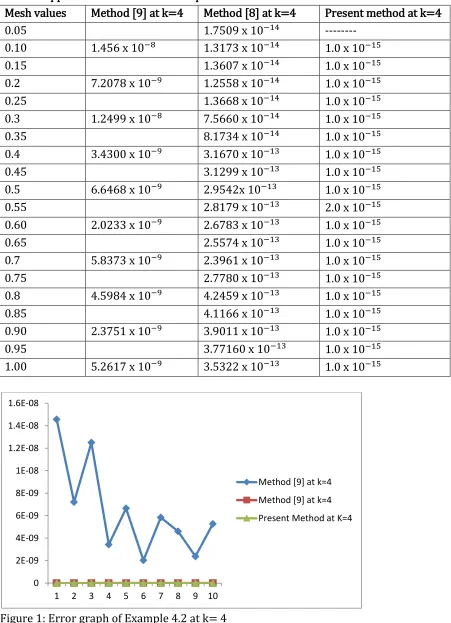
Table 2: Approximate solution of Example 4.2 at k=4
Mesh values Method [9] at k=4 Method [8] at k=4 Present method at k=4
0.05 1.7509 x 10⁻¹⁴ ---
0.10 1.456 x 10⁻⁸ 1.3173 x 10⁻¹⁴ 1.0 x 10⁻¹⁵
0.15 1.3607 x 10⁻¹⁴ 1.0 x 10⁻¹⁵
0.2 7.2078 x 10⁻⁹ 1.2558 x 10⁻¹⁴ 1.0 x 10⁻¹⁵
0.25 1.3668 x 10⁻¹⁴ 1.0 x 10⁻¹⁵
0.3 1.2499 x 10⁻⁸ 7.5660 x 10⁻¹⁴ 1.0 x 10⁻¹⁵
0.35 8.1734 x 10⁻¹⁴ 1.0 x 10⁻¹⁵
0.4 3.4300 x 10⁻⁹ 3.1670 x 10⁻¹³ 1.0 x 10⁻¹⁵
0.45 3.1299 x 10⁻¹³ 1.0 x 10⁻¹⁵
0.5 6.6468 x 10⁻⁹ 2.9542x 10⁻¹³ 1.0 x 10⁻¹⁵
0.55 2.8179 x 10⁻¹³ 2.0 x 10⁻¹⁵
0.60 2.0233 x 10⁻⁹ 2.6783 x 10⁻¹³ 1.0 x 10⁻¹⁵
0.65 2.5574 x 10⁻¹³ 1.0 x 10⁻¹⁵
0.7 5.8373 x 10⁻⁹ 2.3961 x 10⁻¹³ 1.0 x 10⁻¹⁵
0.75 2.7780 x 10⁻¹³ 1.0 x 10⁻¹⁵
0.8 4.5984 x 10⁻⁹ 4.2459 x 10⁻¹³ 1.0 x 10⁻¹⁵
0.85 4.1166 x 10⁻¹³ 1.0 x 10⁻¹⁵
0.90 2.3751 x 10⁻⁹ 3.9011 x 10⁻¹³ 1.0 x 10⁻¹⁵
0.95 3.77160 x 10⁻¹³ 1.0 x 10⁻¹⁵
1.00 5.2617 x 10⁻⁹ 3.5322 x 10⁻¹³ 1.0 x 10⁻¹⁵
Figure 1: Error graph of Example 4.2 at k= 4 0
2E-09 4E-09 6E-09 8E-09 1E-08 1.2E-08 1.4E-08 1.6E-08
1 2 3 4 5 6 7 8 9 10
Method [9] at k=4
Method [9] at k=4
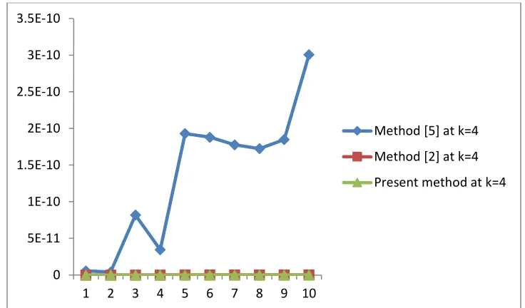
Table 3: Approximate solution of Example 4.3 at k=4
Figure 2: Error graph of Example 4.3 0
5E-11 1E-10 1.5E-10 2E-10 2.5E-10 3E-10 3.5E-10
1 2 3 4 5 6 7 8 9 10
Method [5] at k=4
Method [2] at k=4
Present method at k=4 𝑴𝒆𝒔𝒉 𝒗𝒂𝒍𝒖𝒆𝒔 Method [5] at k=4 Method [2] at
k=4
Present Method at k=4
0.1 5.57443 E (-12) --- --- 0.2 3.946177 E(-12) 2.00 E(-15) ---
0.3 8.183232 E(-11) --- ---
0.4 3.436118 E(-11) 8.00 E (-15) ---
0.5 1.92974 E(-10) 1.20 E (-14) 1.0 E (-15)
0.6 1.87904 E(-10) 1.60 E (-14) 1.0 E (-15)
0.7 1.776835 E(-10) 1.80 E (-14) 2.0 E (-15)
0.8 1.724676 E(-10) 2.30 E (-14) 1.0 E (-15)
0.9 1.847545 E( -10) 2.40 E (-14) 2.0 E (-15)
Table 4: Approximate solution of Example 4.4 at k=4 Mesh
values
Method [9] at k=4
Method [8] at k=4 Present method k = 4
0.05 5.9679 x 10⁻⁴ 4.2826125 x 10⁻⁸
0.10 1.8070 x 10⁻² 1.5485 x 10⁻⁴ 8.27482906 x 10⁻⁸
0.15 8.1938 x 10⁻⁵ 5.581025 x 10⁻⁹
0.20 1.0210 x 10⁻³ 7.5021 x 10⁻⁵ 5.543383 x 10⁻⁹
0.25 1.1954 x 10⁻⁶ 3.7376 x 10⁻¹¹
0.30 1.3225 x 10⁻³ 3.8056 x 10⁻⁶ 2.53 x 10⁻¹³
0.35 1.0512 x 10⁻⁶ 2.00 x 10⁻¹⁵
0.40 4.3646 x 10⁻³ 1.2499 x 10⁻⁶ 1.00 x 10⁻¹⁵
0.45 6.6184 x 10⁻⁷ ---
0.50 7.8860 x 10⁻⁴ 1.9415 x 10⁻⁸ 1.00 x 10⁻¹⁵
0.55 1.0247 x 10⁻⁸ ---
0.60 4.4568 x 10⁻⁴ 9.3785 x 10⁻⁸ ---
0.65 1.4945 x 10⁻⁸ ---
0.70 5.7728 x 10⁻⁴ 4.7574 x 10⁻⁹ ---
0.75 1.3142 x 10⁻⁹ 1.0000 x 10⁻¹⁵
0.80 1.9057 x 10⁻³ 1.5626 x 10⁻⁹ ---
0.85 8.2737 x 10⁻¹⁰ 2.0000 x 10⁻¹⁵
0.90 3.4431 x 10⁻⁴ 2.4271 x 10⁻¹⁰ ---
0.95 1.2804 x 10⁻¹¹ ---
1.0 1.9459 x 10⁻⁴ 1.1724 x 10⁻¹¹ 1.0000 x 10⁻¹⁵
Figure 3: Error graph of Example 4.4 0
0.002 0.004 0.006 0.008 0.01 0.012 0.014 0.016 0.018 0.02
1 2 3 4 5 6 7 8 9 10
Method [9] at k=4
Method [8] at k=4
5.0Discussion of Results
We observed that the Ninth stage Runge-Kutta method performed excellently well with the four problems tested with the method. This shows that our method is good and can be used to solve accurately any model of the form 𝑦′= 𝑓(𝑥, 𝑦), 𝑦(𝑎) = 𝜌. (see Tables 1, 2,3,4 and figures 1,2 and 3)
6.0Conclusion
We want to conclude that the newly block integrator (8) is of uniform order 9, zero stable, consistent and self starting and after reformulating into Runge-Kutta type method, the results obtained from the method converges more excellently than the existing method. (see figures 1, 2 and 3). Although the cost of implementation is high when compare with method [2].
REFERENCES
[1] Badmus A M and Mshelia W D: “Some uniform order block methods for the solution of first order ordinary differential equations” Journal of Nigerian Association of Mathematical Physics, volume 19 pages 149-154. (2011)
[2] Badmus AM and Fatunsi LM A new ninth order Hybrid block integrator for solution of first order ordinary differential equations Asian Journal of Mathematics and Applications volume 2015, article id ama0238, 8 pages
[3] Onumanyi P and Awoyemi D.O, Jator S.N. and Siriseria U.W “New Linear Multistep Methods with continuous coefficients for first order ivps” Journal of Nigeria Mathematics society 13: 37- 51. (1994) [4] Odekunle MR, Adesanya AO, Sunday J “A new block integrator for the solution of initial value problems of
first order ordinary differential equations”International Journal of Pure and Applied Science and Technology (2012)1
[5] Odekunle MR, Sunday J and Adesanya AO: Order six block integrator for the solution of first-order ordinary differential equations. International Journal of mathematics and Soft Computing, volume 3, No1, pages 87-96. (2013)
[6] Chollom JP, Olatunbojun IO, Omagu SA. “A class of A-stable block methods for the solution of ordinary differential equation”. Research Journal of Mathematics and Statistics.;4(2):52-56. (2012)
[7] Fatunla S.O “Block Method for Second Order Differential Equations” International Journal of Computer mathematics. 41: 55-63(1991).
[8] Kwami, A. M A Class of Continuous General Linear Methods for Ordinary Differential Equations, Ph.D. Thesis, Abubakar Tafawa Balewa University, Bauchi, 28 – 57. (2011),
[9] Yakubu, D.G, Onumanyi P and Chollom J P: A new family of general linear methods based on the block Adams-Moulton multistep methods J. of pure and Applied Sciences, 7(1): 98 – 106. (2004),
MSHELIA DW, DEPARTMENT OF MATHEMATICS, UMAR IBN IBRAHIM ELKANAMI, COLLEGE OF EDUCATION, SCIENCE AND TECHNOLOGY, BAMA BORNO STATE
BADMUS AM, DEPARTMENT OF MATHEMATICS, NIGERIAN DEFENCE ACADEMY, KADUNA, NIGERIA