CLIVAR Exchanges No 25 Special issue on: CLIVAR Atlantic

(1)

September 2002

CLIVAR is an international research programme dealing with climate variability and predictability on time-scales from months to decades.

CLIVAR is a component of the World Climate Research Programme (WCRP). Latest CLIVAR News

• New in this issue:

CLIVAR Data Section, see pages 68-73.

• New Version of the CLI-VAR Calendar:

www.clivar.org/calen-dar/. Bookmark the new address and edit/add entries yourself.

• Coming soon: Bookmark

www.clivar2004.org, the official CLIVAR con-ference website.

•

ICPO worldwide: Mike Sparrow works out of his new base in China. See www.clivar.org/or-g a n i z a t i o n / i c p o / sparrow.htm for more information.

Visit our news page: http://www.clivar.org/recent/

Exchanges

Figure 1 from paper ‘Benchmarks for Atlantic Ocean Circulation’ by R. Molinari et al.: Benchmarks being monitored and available on http://www.aoml.noaa.gov/bench-marks/index.html. The paper appears on page 6.

Benchmarks for Atlantic Ocean Circulation

Call for Contributions

We would like to invite the CLIVAR community to submit papers to CLIVAR Exchanges for the next issue.The overarching topic will be on science related to the WOCE / CLIVAR transition. The deadline for this issue is January, 31, 2003.

Guidelines for the submission of papers for CLIVAR Exchanges can be found under: http://www.clivar.org/publications/exchanges/guidel.htm

Special issue on: CLIVAR Atlantic

No. 25 (Vol. 7, No. 3/4)

September 2002

80

60

40

20

0

20

40

60

80

60 20 0

Agulhas Rings & Transport

Gulf Stream Transport

Total water column changes

North Brazil Current Rings Deep Western Boundary

Current Transport

Florida Current Transport

(2)

Editorial

Dear CLIVAR community,

As we reported in out previous issue, the ICPO has a new director. Dr. Howard Cattle has taken over the responsibilities from Dr. John Gould who retired from his CLIVAR job beginning of August. Again, a warm wel-come to Howard and deepest thanks and highest regards to John for leading the ICPO over the past 4 years. Howard is the fourth director of the ICPO, following Dr. Michael Coughlan (1995-97), Dr. Lydia Dümenil (1997-1998) and Dr. John Gould (1998-2002). Together with the CLIVAR Scientific Steering Group, its panels and work-ing groups (currently 12) and the ICPO staff, his chal-lenge will be, to steer and develop CLIVAR further into its fully mature phase.

About 5 years after the publication of the Initial Implementation Plan, CLIVAR has entered its mature phase. National projects are being funded, international coordination is taking place within many parts of the programme and most important, scientific results are being published. For us in the ICPO it is important to monitor the scientific progress of the programme, since this is one of the key parameters to measure the success of the programme, and somehow also a legacy for the community. However it turns out to be much more tricky in many cases to decide what is a CLIVAR publication than for other, more focused programmes like WOCE which, because of their nature, have specific national grants which are referred to. Such acknowledgement will clearly be made if there is indeed a nationally funded programme for CLIVAR (and such programmes do ex-ist in some countries). But acknowledgement may also to some extent be a cultural issue in terms of making the community itself feel it is a part of a programme which it is naturally appropriate to refer to, irrespective of fund-ing lines. This is clearly an issue which CLIVAR as a pro-gramme needs to work on, but it would be helpful if authors of CLIVAR-relevant papers could consider if a reference to CLIVAR is appropriate.

To get a broader overview of what is published within the CLIVAR related science, we have started to collect the titles of CLIVAR related publications of about a dozen peer-reviewed journals and provide this infor-mation on our website, along with links to abstracts, and some kind of indication about the relevance to specific parts of CLIVAR. This is by no means an objective and comprehensive approach but it provides a tool to moni-tor the progress of the programme. Please feel free to visit: http://www.clivar.org/publications/journals/ literature.htm. We will try to maintain and extend this service in the future.

Another tool to demonstrate the progress and the achievements of the programme has been our newslet-ter. During the first years, it was mainly a

communica-tion forum reporting about the progress in building up the organizational and programmatic structure of CLI-VAR. Shortly after the publication of the Initial Imple-mentation Plan and CLIVAR Conference we changed the scope of the newsletter and invited the community to report about scientific progress on topics related to CLI-VAR. Certainly, not everybody is in favour of this ap-proach. Because the articles published in Exchanges are not reviewed they form part of grey literature and not every contribution might be well balanced and as of high quality as papers are in the peer-reviewed literature. We are taking this risk into account and the response to our calls for contributions has proved the wide interest of the community to have and use this forum. If controver-sial discussions about papers in Exchanges arise, we are happy to expose the community to this and we are will-ing to publish letters to the editor as we have done in the past. We feel that different views are part of living and developing science and these discussions often contrib-ute to scientific progress.

Until today, we have published more than 120 sci-entific articles in Exchanges and this 25th_{issue is a very} special one. Not only, because it is a double number 3/4 2002, but we have never received as many contributions as we have for this issue. Of course, the overarching theme CLIVAR Atlantic is broad and encompasses many research topics within CLIVAR, but the response has also shown that we are on the right track with Exchanges. We think that a wide overview about CLIVAR related research within the Atlantic has been provided.

In addition, we are starting a new regular section on CLIVAR data and data management in Exchanges. We like would to report new efforts within this area as well to provide information about existing data sets, data centres and data management efforts within WCRP and other relevant programmes. We encourage submissions of contributions relevant to this topic.

As many of you know, WOCE is coming to a con-clusion at the end of this year. The final WOCE confer-ence in San Antonio, Texas, USA will highlight this very successful WCRP programme in a very comprehensive way. In order to honour the accomplishments of WOCE and the legacy to CLIVAR we will dedicate the next is-sue of Exchanges (1/2003) on the WOCE-CLIVAR tran-sition. Although we will specifically approach a number of scientists for contributions, papers submitted by the community are very welcome. The deadline for submis-sions is January 31, 2003.

We hope that you will enjoy this very special issue of Exchanges.

(3)

Dear CLIVAR community,

I am grateful to Andreas Villwock for his words of welcome above and like him must firstly pay tribute to John Gould for all he has done for CLIVAR during his time as Director of the ICPO. I have taken over a well-run office and an enthusiastic team and I only hope I can maintain the momentum. As one person emphasised, at the SSG in Xian, China this year, I have some big shoes to fill. The regard in which John is held is, I am sure, reflected in the very warm welcome everyone has given me on my entry into the CLIVAR world, a welcome I have been much encouraged by. John is still close by in the office across the corridor helping to bring WOCE to its conclusion. Having his advice and wisdom at hand is very welcome at this (very steep) stage of my learning curve.

As Andreas has said, CLIVAR is now in its ma-ture phase and, as I am learning, there are many and varied initiatives underway under the CLIVAR banner. Ultimately, CLIVAR exists as a project of WCRP to set the agenda for and to facilitate international collabora-tion in research on climate variability and predictability. This is, of course carried out through the Scientific Steer-ing Group and its panels and workSteer-ing groups and it is a primary role of the ICPO to assist with the practical im-plementation of their work. I am looking forward to working with others in the ICPO as well as all in the CLIVAR panels and working groups and the wider com-munity on the variety of CLIVAR activities and initia-tives.

It is clear that there will be many challenges ahead. A key outcome of the meeting of the Joint Scientific Com-mittee (JSC) for WCRP when it met in Hobart in March 2002 was a proposal for an overall WCRP banner on pre-dictability. This is an issue of which lies at the heart of CLIVAR (indeed sitting within its very title). CLIVAR has the natural lead within WCRP for this therefore, but

there is a need to clarify the issues and CLIVAR has a key contribution to make to formulate the way ahead, together with the other WCRP projects.

WOCE is, as I have mentioned, coming to an end. It has done a wonderful job in providing us amongst other things with an unparalleled database of ocean cli-mate. For the future, however, the issue of monitoring the variability of the ocean on climate time-scales and the role CLIVAR has to play as the lead within WCRP for this is a key one, as John Gould has emphasised on more than one occasion. With the exception of its mod-elling groups, the CLIVAR panel structure itself largely addresses the variability of the climate system on regional and basin-scale. One of the concerns of the JSC at its last meeting was the need for us to better articulate how these contribute to and build into an overall global picture. We need to think how we best do this. Another issue for CLIVAR, described at the last SSG meeting as “getting your arms around the data elephant” is that of CLIVAR data management and how we go about it, This is an area of concern not only to CLIVAR but to WCRP as a whole. From a CLIVAR perspective, it is one that needs to be addressed with the help of all the panels and work-ing groups as well as the ICPO.

These are but a few examples of the many chal-lenges facing us. An event still a little way off, but one which will soon become larger in our minds is that of the First International CLIVAR Science Conference, to be held in Baltimore, USA from 21-25 July 2004. Plan-ning for this exciting event is already well underway. The Conference will be a real opportunity for us to as-sess progress in CLIVAR science against our implemen-tation plan and to consider the directions CLIVAR should take in the second half of the decade.

So, there is much work to be done and I am look-ing forward to our future involvement together. Whilst I am no stranger to WCRP projects, I trust you will bear with me as I settle into my new role. At the same time please provide me with appropriate advice and correc-tion whenever you feel I am taking the wrong turn. I will always be pleased to receive and hopefully to re-spond positively to comments on CLIVAR, its structure and activities and in particular the role of those of us at the ICPO. We are here to be as helpful as we can.

(4)

M. Visbeck (chair)1, David Marshall2 and the

CLIVAR-Atlantic Implementation Panel

1_{Lamont Doherty Earth Laboratory, Palisades, NY,}

USA

2_{University of Reading, Reading, UK}

corresponding e-mail: [email protected]

Introduction

Our panel looks after the implementation of CLI-VAR in the Atlantic sector with an emphasis on three phenomena: Tropical Atlantic Variability, the North At-lantic Oscillation, and changes in the ocean’s meridional overturning. The primary goal is to improve our descrip-tion and understanding of those modes of variability and then explore to what degree they might be predictable on seasonal to decadal time scales. An important objec-tive is to study the interaction between those phenom-ena and large scale forcings of the global climate system such as due to El Niño and/or anthropogenic climate change.

The CLIVAR Atlantic panel has met approximately annually during the last 3 years. In December 2000 the focus was on implementation issues associated with the North Atlantic Oscillation in conjunction with the Chapman Conference (Visbeck et al., 2001). In Septem-ber 2001 we reviewed ongoing and planned activities in the tropical Atlantic following a CLIVAR sponsored workshop on the subject (Garzoli, 2001). This year’s meeting (July 2002 in Bermuda) focused on CLIVAR ac-tivities and plans regarding the oceans meridional over-turning circulation. A number of invited experts and rep-resentatives from WGCM and WGOMD were present to enrich the discussions. A brief review on the MOC and related CLIVAR activities is given below.

Atlantic Meridional Overturning Circulation: Issues for Models and Observations

The Meridional Overturning Circulation (MOC) in the Atlantic transports approximately 20 Sv of warm water northward in surface layers, with compensating southward flow at depth. Associated with this overturn-ing is a northward heat transport, peakoverturn-ing at about 1PW in the subtropical North Atlantic. It is widely (though not universally) accepted that this heat is an important factor in determining surface air temperatures over much of the North Atlantic Sector. On long time scales the strength of the MOC is dominated by this thermohaline driving (a balance between surface buoyancy loss in high latitudes and buoyancy gain by diapycnal mixing in the tropical oceans and/or the Southern Ocean). In contrast, on interannual and shorter time scales wind-driven Ekman cells dominate its variability. This mix of forcing poses significant challenges for sustained observations.

A significant number of projections of greenhouse-gas induced climate change over the next century indi-cate a weakened MOC in the North Atlantic due to fresh-ening of the subpolar ocean, although there is little con-sensus on the rate and magnitude of the projected change (IPCC, 2001). A key issue is therefore to understand the spread in these predictions, and to determine whether this is indicative of shortcomings in the models or an inherent lack of predictability in the response of the MOC, and to attempt to reduce the uncertainties. Obser-vations reveal consistent evidence of long-term changes in the properties of the overflows and in convectively renewed water masses in the Labrador Sea; the present observational network seems inadequate, however, to directly determine whether the strength of the MOC is in the process of decreasing by 10-20% as anticipated. In addition, even with perfect observations it would be dif-ficult to detect an MOC climate change signal without an adequate understanding of the natural variability of the MOC. This argues both for improved understand-ing of the fundamental processes controllunderstand-ing the MOC and its variability, such as can be achieved through theo-retical and modelling studies, and for efforts to quantify the natural variability of the MOC.

The thermohaline circulation responds to surface forcing on a range of time-scales. The initial dynamical adjustment occurs via the propagation of Kelvin waves and Rossby waves on the time-scale of months-decades; in contrast thermodynamic equilibrium is approached over several centuries. Thus, while eddy-permitting models can be used to study the initial dynamical ad-justment of the thermohaline circulation, it is still neces-sary to employ relatively coarse-resolution models in order to study the time-mean circulation and anthropo-genic climate-change scenarios. These latter models not only fail to resolve the geostrophic eddy field, but also fail to adequately resolve the narrow boundary currents and their recirculations within which most of the heat transport occurs; thus the results of such coarser models need to be treated with caution. Even in eddy-permit-ting models, there remain several important processes that require careful parameterisation such as shelf and open-ocean convection, overflows and sea-ice. Models can be particularly sensitive to these parameterisations, for example Dengg and Böning (2002) have found that subtle changes in the density of the water flowing over the Denmark Straits can lead to dramatic changes in MOC downstream due to entrainment in the overflows.

(5)

latitude North Atlantic, or “pulled” by Ekman transports in the Southern Ocean and/or diapycnal mixing in the ocean interior, temporal anomalies in MOC are likely to be confined to the hemisphere in which they are gener-ated on decadal and shorter time-scales. However the Atlantic MOC may still have a rapid global impact. Dong and Sutton (2002) have performed a provocative calcu-lation in which the thermohaline circucalcu-lation is abruptly halted by an impulsive reduction in high-latitude salin-ity. Circulation anomalies are found in the tropical At-lantic within 6 months via the propagation of a Kelvin wave. These anomalous currents modify the cross equa-torial Atlantic SST gradient (with cooling in the North Atlantic) and shift the mean position of the ITCZ south-ward; the latter in turn leads to a global atmospheric re-sponse within seven years. While a somewhat extreme scenario, this experiment serves as a useful reminder that the response of the climate system to a change in high latitude ocean conditions is likely to involve a combina-tion of oceanic and atmospheric teleconneccombina-tions, with coupling most likely occurring in the tropical belt. In the absence of an abrupt shutdown, natural variations in MOC are likely to be significantly smaller, but still pos-sibly important. For example, recent observational analy-ses (Landsea et al., 1999) have noted a link between At-lantic multidecadal SST variations and hurricane activ-ity. To the extent that these multidecadal fluctuations in SST are related to variations in the MOC, this points to a potentially important role for the MOC in modulating Atlantic hurricanes.

A further motivation for improving our ability to understand and model the dynamical response of the ocean to surface forcing is to aid in the design and inter-pretation of observations of the MOC. A substantial port-folio of observations targeting the Atlantic MOC is now taking shape. This includes: various activities under the ASOF programme aiming to measure fresh water fluxes between the Arctic and Atlantic (see Dickson and Boscolo, 2002); the basin scale hydrographic programme ( h t t p : / / c l i v a r - s e a r c h . c m s . u d e l . e d u / h y d r o / hydro_table.asp); a series of Labrador Sea/Grand Banks moored arrays (IfM Kiel, Schott et al.); transport meas-urements in the Florida straits; the MOVE array at 16o_N (IfM Kiel, Send et al.); and the tropical Atlantic surveys

conducted by research labs in the USA, France and Ger-many. In addition there are a number of proposed ef-forts including an array of three sections to monitor the communication of deep MOC anomalies along the shelf between Grand Banks and Cape Cod (Hughes, Marshall, Williams); a line at 39o_{N (WHOI, Toole et al.); a proposed} array across 26o_{N (SOC, Marotzke et al.) which, together} with the ongoing efforts should provide data from which a time series of MOC observations could be constructed. However, it might be best to include satellite data of sea surface height and temperature; in situ data from the PIRATA array, XBT’s and the emerging ARGO profiles (see also http://www.clivar.org/organization/atlantic/ IMPL/index.htm) to obtain a basin wide synthesis us-ing a variety of methods includus-ing 4 dimensional data assimilation (Stammer et al., 2002). In the South Atlantic the observational data base is thinner, and as a result, our knowledge of the role of the South Atlantic in the coupled climate system is less certain. Efforts are underway to identify the climate variability in the re-gion and the broad scale and targeted ocean observa-tions needed to increase our understanding. A workshop is planned for early 2003 to initiate this activity.

In summary CLIVAR is well underway in the At-lantic sector. A significant number of national and inter-national observational, modelling and synthesis pro-grammes exist in support of CLIVAR objectives.

References

Dengg, J., and C. Böning, 2002: Effects of Denmark Strait Over-flow on the large-scale circulation in a numerical model of the North Atlantic, J. Phys. Oceanogr., to be submit-ted.

Dickson, R., and R. Boscolo, 2002: The Arctic-Subarctic Ocean Flux Study (ASOF): Rational, Scope and Methods. CLI-VAR Exchanges, 25, 64.

Dong, B.-W., and R.T. Sutton, 2002: Adjustment of the coupled ocean-atmosphere system to a sudden change in thermohaline circulation. Geophys. Res. Lett., submitted. Garzoli, S., 2001: Workshop on tropical Atlantic variability.

CLI-VAR Exchanges, 22, 33-35.

IPCC, 2001: Climate Change 2001: The Scientific Basis. In: Con-tribution of Working Group I to the Third Assessment Re-port of the Intergovernmental Panel on Climate Change, Houghton, J.T., Y. Ding, D.J. Griggs, M. Noguer, P. van der Linden, X. Dai and K. Maskell, Eds., Cambridge University Press, Cambridge, UK.

Johnson, H.L., and D.P. Marshall, 2002: Localization of abrupt change in the North Atlantic thermohaline circulation. Geophys. Res. Lett., 29, in press, 10.1029/2001GL014140. Landsea, C.W., R.A. Pielke, Jr., A.M. Mestas-Nunez, and J.A. Knaff, 1999: Atlantic basin hurricanes: indices of climate change. Climatic Change, 42, 89-129.

Stammer, D., C. Wunsch, I. Fukumori, and J. Marshall, 2002: State estimation improves prospects for ocean research. EOS, Transactions American Geophysical Union, Vol. 83, No. 27, p. 289, 294-295.

Visbeck, M., J.W. Hurrell, and Y. Kushnir, 2001: First Interna-tional Conference on the North Atlantic Oscillation (NAO): Lessons and Challenges for CLIVAR. CLIVAR Exchanges, 19, 24-25.

(6)

Robert L. Molinari, Roberta Lusic, Silvia L. Garzoli, Molly O. Baringer and Gustavo Goni

NOAA/AOML, Miami, FL, USA

Oceanographers frequently decompose the total oceanic circulation into two components: a wind-driven component existing primarily in the horizontal plane and a thermohaline-driven component existing primarily in the vertical plane (also called the meridional overturn-ing circulation, MOC). Although this decomposition is a simplification of the dynamics of the motion in the ocean (the two components are not separable in the complete equations of motion), it provides a framework for de-scribing responses of the ocean to different surface forc-ing functions. Numerical modellforc-ing, paleoclimate and observational studies indicate that both the wind-driven and thermohaline circulation can play an important role in longer-term (greater than decadal) climate variability. The U.S. National Oceanic and Atmospheric Adminis-tration addresses both components to satisfy its missions of detecting, attributing and forecasting long-term cli-mate change. We contribute to NOAA’s mission by de-veloping and providing observational benchmarks (i.e., indices) for various components of the wind-driven cir-culation (hereinafter WDC) and MOC in the Atlantic Ocean.

Many early NOAA programmes (e.g. STACS, ACCP) were searching for indices of critical North At-lantic WDC and MOC features to monitor. Although not originally NOAA programmes, other studies have con-sidered the contribution of southern hemisphere features to the MOC. For continuity of the upper layer limb of the MOC, exchanges are required: from the Indian Ocean to the South Atlantic; across the South Atlantic; and across the equator. The inter-ocean exchange takes place through the Benguela/Agulhas system, south of South Africa. The Agulhas Current at its retroflection sheds energetic rings that carry salt and warm water into the South Atlantic. Satellite altimetric measurements have been calibrated to provide estimates of the transport of the Agulhas Current and the separated rings. The exten-sion of the Benguela Current brings the Indian Ocean waters to the central South Atlantic as it flows northwestward in the South Atlantic subtropical gyre.

The pathways of the upper limb MOC transport are then complicated by the wind-driven circulation fea-tures along the western boundary and the interior tropi-cal Atlantic (i.e., equatorial upwelling, off-equatorial down welling, zonal currents), that provide obstacles for this limb to move from the South Atlantic to the North Atlantic. Currently, there is insufficient understanding and data to identify these pathways precisely. However numerical models do provide some initial guidance.

Using an eddy-resolving numerical circulation model, Fratantoni et al. (2000) concluded that 14 Sv of upper limb MOC flow is partitioned among three pathways connecting the equatorial and tropical wind-driven gyre: a frictional western boundary current accounting for 6.8 Sv; a diapycnal pathway involving wind-forced equato-rial upwelling and interior Ekman transport, 4.2 Sv; and North Brazil Current (NBC) rings shed at the NBC ret-roflection, 3 Sv. The results of an AOML, university ob-servational programme indicate that previous estimates both in the numbers of rings per year and in their contri-bution to hemispheric exchanges were low. Based on the results of this work, a monitoring strategy is being de-veloped to monitor ring formation and propagation.

Both the intensity of the subtropical gyre and a component of the warm upper level poleward flow in the North Atlantic are being monitored by submarine cable observations in the Straits of Florida. Similarly, the characteristics of the cold deep return flow are being tracked by research vessel transects across the DWBC east of the Bahamas. In the North Atlantic Ocean, time-series of both the upper layer temperature structure within the subtropical gyre and total water column changes across the basin are being maintained.

The recent history of these and other components of the MOC and WDC motions are characterized by data collected over the past 10 to 50 years. These benchmarks are designed to serve several purposes. Independently these benchmarks serve as indices for (1) the intensity of various components of the MOC and WDC, thereby pro-viding alerts for dramatic changes in these features and (2) verification of the ability of GCM’s to simulate the ocean’s role in climate variability. Collectively, when as-similated into GCM’s they will provide global bench-marks for detection and attribution of climate change. All the benchmarks presently available are shown in Fig. 1 (page 1). We will now describe a few of these indices; where sufficient data are available we provide a descrip-tion of the characteristics of various scales of variability.

1. Agulhas Current

(7)

Agulhas Current and ring shedding characteristics

After turning to the west, the circulation of this current turns or retroflects back to the east between 15 and 25o_{E (Fig. 2, upper panel). The net westward} baro-clinic transport across a TOPEX/POSEIDON groundtrack (light grey line in the top panel of Fig. 2) is estimated using altimetry-derived sea height anomaly and historical hydrographic data within a two-layer re-duced gravity scheme.

• Mean annual transport and number of rings shed: The mean annual transport of the Aguhlas Current from the coast to 40°S above the 10°C isotherm is 15.7 ± 1.5 Sv, with a maximum of 23 ± 1.5 Sv in 1997 and a minimum of 13 ± 1.5 Sv in 1993. The number of rings shed at the retroflection is between 4 and 7 per year and the transport of the rings varies between 0.8 and 2.4 Sv.

• Interannual signal: Strong interannual variability in the transport time series is primarily related to ring shedding (Fig. 2, center panel).

• Annual signal: The altimeter-derived Agulhas trans-port shows no apparent seasonal signal (Garzoli and Goni, 2000), contrary to previous numerical model results (Matano et al., 1998).

2. North Brazil Current

The North Brazil Current is a western boundary current in the tropical Atlantic that transports upper ocean waters across the equator. Particularly during sum-mer and fall, the NBC retroflects from the coast at 6° to 7°N and feeds the North Equatorial Countercurrent and North Equatorial Undercurrent. During this retroflection phase large anticyclonic rings are shed. These features then move northwestward toward the Caribbean Sea, roughly paralleling the South American coastline. As part of the NBC Ring study, an analysis of altimetric data was made (Goni and Johns, 2001). Using a two-layer reduced gravity model, sea height anomaly was converted into upper layer thickness. The thickness maps are used to infer the NBC rings formation and propagation. Analy-sis of the historical altimetric record indicates that ring shedding is nearly a factor of two greater than previ-ously estimated even though the altimeter does not track all the rings formed at the retroflection, (Garzoli et al., 2002).

North Brazil Current rings characteristics

• Transport resulting from mean annual ring shedding: The estimated yearly mass transported by rings is 9 Sv.

• Interannual variability: The available time series of ring shedding derived from the altimeter is shown in Fig. 3.

• Annual cycle: There are insufficient data to determine if there is an annual signal in ring generations. How-ever, the analysis of the IES data obtained during the North Brazil Current ring experiment (Garzoli et al., 2002) indicates that there is no seasonality.

3. Florida Current Transport

The Florida Current (FC) is the western boundary current for the subtropical gyre of the North Atlantic. In addition, to transporting water masses originating in the northern hemisphere, the FC advects water from the southern hemisphere that has crossed both the equator and the North Atlantic’s tropical/subtropical gyre boundary. Ultimately, a portion of the FC transport be-comes entrained in the subpolar gyre where it contrib-utes to the formation of the deeper water masses. Begin-ning in the early 1980’s, submarine cable observations of voltage differences across the Straits have been cali-brated with direct current data to estimate FC transport.

Florida Current characteristics

• Mean annual transport: The mean annual transport of the Florida Current at 27o_{N over the cable record is} 32 Sv. Earlier data collected at 26o_{N during the late} 1960’s early 1970’s observed a mean annual trans-port of 30 Sv (Niiler and Richardson, 1973). Johns et al., (1999) computed a mean annual transport through the NW Providence Channel (located be-tween the two transport sections) of about 1 to 2 Sv. Thus over the past 30+-years the mean annual trans-port of the Florida Current appears stable.

Fig. 2: (top) Schematic of the Agulhas Current retroflection. (center) Baroclinic transport from the surface to the 10°C iso-therm across a selected TOPEX/Poseidon altimeter ground track from the coast to 40°S. (light grey line in top panel). (centre) Baroclinic transport between 1993 and 1995 showing a strong correspondence between ring shedding (circles) and maximum transport values (bottom).

YEAR

1993 1994 1995

0 10 20 30 40

Upper Layer Transport (Sv)

YEAR

1993 1994 1995 1996 1997 1998 1999 2000 0

10 20 30 40

Upper Layer Transport (Sv)

40˚S 30˚S

(8)

• Decadal signals: A smoothed version of the 20-year series is shown in Figure 4. On decadal time-scales, the variability is less than 4 Sv (10-15% of the mean annual signal). This signal in FC transport is visually correlated with a NAO-index with similar time-scales (Fig. 4).

• Annual signal: Using the 1960/1970’s data, (Niiler and Richardson, 1973) estimated an annual signal for FC transport. Largest transports were in the summer and minimum, in the fall. The amplitude of the an-nual signal was about 3 SV. However, (Behringer and Larsen, 2001) found a larger semi-annual com-ponent in the more recent transport data than ob-served in the earlier records.

4. Lower Layer

The Deep Western Boundary Current (DWBC) provides the main conduit for waters formed in the subpolar and polar Atlantic to the South Atlantic and then on to the other ocean basins. As surface forcing func-tions change in the formation regions for the DWBC water masses, the characteristics of the water masses will vary downstream. Tracking these changes provides a benchmark for evaluating model simulations of the ad-vective times from the formation regions. For example, a water mass formed in the Labrador Sea (LSW) is

advected in the DWBC to 26.5o_{N, east of Abaco Island,} the Bahamas. Time series of the characteristics of LSW at Abaco provide a benchmark for present day advec-tive time-scales from source to subtropical western boundary.

Lower layer characteristics

Decadal Signal: Temperature and salinity characteristics at the depth of LSW in the DWBC at 26.5o_{N are shown in} Fig. 5 (page 35). Late-90 cooling and freshening can be correlated to changes in the characteristics of LSW at its formation region. The comparison indicates the arrival of LSW at Abaco some 8 to 10 years after formation in the Labrador basin. These advective times are somewhat shorter than previously hypothesized but consistent with other observations obtained in the central subtropical and eastern mid-latitude Atlantic (Molinari et al., 1998).

References

Baringer, M.O., and J.C. Larsen, 2001: Sixteen years of Florida Current transport at 27°N. Geophys. Res. Lett., 28, 3179-3182.

Fratantoni, D.M., W.E. Johns, T.L. Townsend, and H.E. Hurlburt, 2000. Low-Latitude Circulation and Mass Transport Pathways in a Model of the Tropical Atlantic Ocean. J. Phys. Oceanogr., 30 (8), 1944-1966.

ND J F M A M J J A S O N D J F M A M J

600 800 1000 1200 1400 1600 1800 2000 o o oooo oo ooo oo o ooo o o ooo oo o o o o o oo o o oo o oo oo o o oo o o ooo oo oo o o o o ooo ooo o ooo o o o oo oo ooo oo o o o oo oo oo ooo o o o o ooo ooo o o oooooooo o oo ooo oo oo o oooooooo o o o ooo o oo o oo oo o o o o o o oo oooo oo oooo oo ooooo o oooo o o o o o o oo oo o ring 1 ring 2

ring 3 ring 4

ring 5 ring 6 ring 7 ring 8 ring 9 ring 10 ring 11

Northern Penetration of the Retroflection

Distance to 0

o N, 40 o W (km)

Time (month)

1998 1999 2000

(9)

Garzoli, S.L., Q. Yao, and A. Ffield, 2002: North Brazil Current rings and the variability in the latitude of retroflection. In: Interhemispheric Water Exchange in the Atlantic Ocean, G. Goni and P. Malanotte-Rizzoli (Eds.), Elsevier Sci-ence, submitted.

Garzoli, S.L., and G. Goni, 2000: Combining altimeter observa-tions and oceanographic data for ocean circulation stud-ies. In: Satellites, Oceanography and Society, Halpern, D., (ed.) Elsevier Science B. V., 79 -97.

Goni G., and W.E. Johns, 2001: A Census of North Brazil Cur-rent Rings Observed from TOPEX/POSEIDON Altimetry: 1992 – 1998. Geophys. Res. Lett., 28, 1-4. Hurrell, J.L., 1995: Decadal Trends in the North Atlantic

Oscil-lation: Regional Temperatures and Precipitation. Science, 269, 676.

Johns, E., W.D. Wilson, and R.L. Molinari, 1999: Direct obser-vations of velocity and transport in the passages be-tween the Intra-Americas Sea and the Atlantic Ocean, 1984-1996. J. Geophys. Res., 104, 25805-25820.

Matano, R.P., C.G. Simionato, W.P. de Ruijiter, P.L. van Leeuween, P.T. Strub, D.B. Chelton, and M.G. Schlax, 1998: Seasonal variability in the Agulhas retroflection region. Geophys. Res. Lett., 25, 4361-4364.

1982

1984

1986

1988

1990

1992

1994

1996

1998

25

30

35

40

1982

1984

1986

1988

1990

1992

1994

1996

1998

25

30

35

40

Florida Current Transport, Sv (10

6

m

3

s

-1

)

1982

1984

1986

1988

1990

1992

1994

1996

1998

30

32

34

c)

b)

a)

Fig. 4: Time series of Florida Current transport inferred from the cable voltages including (a) the daily transport values, (b) the monthly average transport, and (c) the two year running means of the daily transport values (solid line). Panel (c) also includes a monthly mean NAO index (Hurrell, 1995) (dashed line). Panel (a) includes in situ observations of Florida Current transport obtained on small boat cruises (solid circles).

Molinari, R.L., R.A. Fine, W.D. Wilson, R.G. Curry, J. Abell, and M.S. McCartney, 1998: The arrival of recently formed Labrador Sea Water in the Deep Western Boundary Current at 26.5o_N._{Geophys. Res. Lett}_.,₂₅_{, 2249–2252.}

(10)

Juliet Hermes1, Chris J.C. Reason1, Johann R.E.

Lutjeharms1_{, and Arne Biastoch}2

1_{EGS and Oceanography Departments, University of}

Cape Town, Rondebosch, South Africa

2_{Institut für Meereskunde, Universität Kiel}

Kiel, Germany

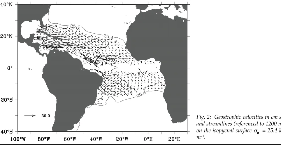
Indian-Atlantic ocean water exchange south of Africa is an important component of the global thermohaline circulation. Evidence exists that variabil-ity in these exchanges, on both meso- and longer time scales, may significantly influence weather and climate patterns in southern Africa (e.g., Walker, 1990; Reason and Mulenga, 1999; Rouault et al., 2002). Observational estimates of the rate of mass and heat exchange between these oceans have varied and it has been difficult to verify these in any reliable manner. Results to date have been comprehensively reviewed by De Ruijter et al. (1999). Model based diagnostics of the inter-ocean fluxes are essential. As a first step in this direction, a model de-signed especially for the Agulhas system has been used in this initial study of the inter-ocean volume and heat fluxes and their seasonal to interannual variability (more details can be found in Reason et al., 2002).

Results were obtained from a 12 yr post spin up integration of the regional eddy permitting model, Agape of Biastoch and Krauß (1999) (more details can be found on http://www.ifm.uni-kiel.de/fb/fb1/tm/research/ woce/agulhas/agape.html). The heat and volume fluxes are calculated from 5 year statistics after the spin-up.

The annual mean heat transport and net surface heat flux along various sections are plotted in Fig. 1.

There is a net westward transport through 20o_{E of 0.84} PW (Fig. 1) but this ranges from 1.3 PW westwards dur-ing the sprdur-ing of year 32 to only about 0.35-0.5 PW west during each summer/autumn (Fig. 2). Even though the volume transport is sometimes eastwards, the net heat transport is always west into the SE Atlantic, due to the Agulhas Current water being much warmer than the water further south along this section. At 5o_{E the Agulhas} transport is returned by the retroflection so that there is an eastward transport of 0.02 PW on the annual mean. However, eastward transport only occurs in summer and autumn, during winter and spring this transport is west-wards. The model estimate of 1.03 PW flowing north along 35o_{S is larger than previous hydrographic estimates} (0.02-0.47 PW – Gordon (1985)) and model calculations (0.51 PW – Thompson et al. (1997) and 0.6 PW – Semtner and Chervin (1992)), but these models omitted factors such as the Indonesian Throughflow and the Mozam-bique Channel flow.

In terms of the volume transport, the annual mean transport into the SE Atlantic is around 2.9 Sv through 20o_{E and about 15.5 Sv through 35}o_{S. Much of this flow} re-circulates so that only about 0.3 Sv escapes into the SE Atlantic west of 5o_{E. Substantial variability does} oc-cur on monthly through to interannual time scales as shown in Figs. 2 and 3. In terms of volume flux, although the mean annual transport through 20°E is always to the west, it can vary with as much as 12 Sv flowing east from the SE Atlantic into the South Indian ocean during the summer of year 34 to almost 16 Sv west into the SE At-lantic during the winters of years 31 and 34. This corre-sponds to an annual mean heat transport of 0.84 PW going westward through 20°E (Fig 2a), but ranging from as much as 1.3 PW west into the SE Atlantic during spring of year 32 to only about 0.35-0.5 PW west during each summer/autumn (Fig. 2b). Note that figure 3a and b cover the latitude band of Fig. 2 in two separate parts.

The fluxes discussed above refer to both the eddy component and the mean current (includ-ing Agulhas r(includ-ings). Estimates of the eddy variabil-ity (not rings) were made and reveal that along the section at 20o_{E there is a net west transport} into the South Atlantic of 0.12 PW, as compared to the total westwards transport integrated along this section of 0.84 PW. These results suggest that in the model it is eddy variability associated with the southern Agulhas, and not rings, which sig-nificantly contribute to the heat transport into the South Atlantic.

Time series and spectra of the heat and vol-ume transports at various locations in the region, obtained from years 31-43 of the integration were calculated and are shown in Fig. 3 a-c. Fig. 3a (sec-Inter-ocean Fluxes south of Africa in an Eddy-permitting Model

Fig. 1: The annual mean total heat transport (PW) and net surface heat flux (contour interval 10 Wm-2_{) averaged over years 31-35 of the} model integration.

0 5 10 15 20 25 30 35 40 45 50

50 45 40 35 30

LONGITUDE

LATITUDE

SURFACE (W/m**2) AND DEPTH AVERAGED HEAT FLUXES (PW)

10

80

2₀

140 60

50 1 0 40 10

30 ₈₀

20

30

110 20

50

20

40

10

80

40

0

1.025

2.926

0.219

0.142

0.836

2.245

(11)

Fig. 2: Upper panel: Monthly mean heat transport (PW) (bold line) along 20o_{E between 45-35}o_{S together with the maximum} (upper line) and minimum (lower line) values and one stand-ard deviation above and below the mean (stippled lines). Lower Panel: time series of this transport for years 31-35 of the integration.

-200 -150 -100 -50 0

Volume flux (Sv)

Years

-6 -5 -4 -3 -2 -1

Heat flux (PW)

Years

0 0.01 0.02

104

102

100 12 6 3 2 Months

Spectral energy

Frequency in cycles per day

20o_{E BETWEEN 35}o_{TO 40}o_S

0 0.01 0.02

104

102

100 12 6 3 2 Months

Spectral energy

a)

33 35 37 39 41 43

0 50 100 150

Volume flux (Sv)

Years

1 2 3 4 5 6

Heat flux (PW)

Years

0 0.01 0.02

104

102

100 12 6 3 2 Months

Spectral energy

0 0.01 0.02

104

102

100 12 6 3 2 Months

Spectral energy

b)

33 35 37 39 41 43

100 50 0 50

Volume flux (Sv)

Years

3 2 1 0 1

Heat flux (PW)

Years

0 0.01 0.02

104

102

100 12 6 3 2 Months

Spectral energy

0 0.01 0.02

104

102

100 12 6 3 2 Months

Spectral energy

c)

33 35 37 39 41 43

Fig. 3: Time series and normalised spectra of total heat and volume fluxes from years 31-43 of the model integration at (a) 20o_{E between 35 and 40}o_{S, (b) 20}o_{E between 40 and 45}o_{S and} (c) 5o_{E between 35 and 40}o_{S. The diamonds indicate the 95 %} confidence interval.

tion of Agulhas Current) displays a peak at around 3 months, this is most likely to be associated with Agulhas ring shedding which occurs on this timescale. The semi-annual signal seen in Fig. 3b appears to be a feature of the Agulhas and Agulhas Return Current. Spectral en-ergy at this timescale does not show up on the trans-ports averaged along other sections (e.g. at 5o_{E). Whether} this signal is derived from the Southern Hemisphere semi-annual oscillation in mid- to high latitude winds and surface pressure, or from that in the South Equato-rial and East Madagascar Currents (Matano et al., 2002) is yet to be determined. Fig. 3c displays significant events that occur in the 5o_{E section that do not occur in the} up-stream sections. These result from seasonal variability in the longitudinal position of the Agulhas retroflection zone, which directly influences this section and leads to the dominating 12 month spectral peak. Meridional shifts also occur, contributing to the shifts in transport sign.

(12)

Reason, C.J.C., J.R.E. Lutjeharms, J. Hermes, A. Biastoch, and R.E. Roman, 2002: Inter-ocean fluxes south of Africa in an eddy-permitting model. Deep-Sea Res., in press. Reason, C.J.C., and H. Mulenga 1999: Relationships between

South African rainfall and SST anomalies in the South-west Indian Ocean. Int. J. Climatol., 19 (15), 1651-1673. Rouault, M., S.A. White, C.J. C.Reason, J.R.E. Lutjeharms, and

I. Jobard, 2002: Ocean-atmosphere interaction in the Agulhas Current and a South African Extreme weather event. Weather and Forecasting, 17 (4), 655-669.

Semtner Jr., A.J., and R.M. Chervin, 1992: Ocean general circu-lation from a global eddy-resolving model. J. Geophys. Res., 97, 5493-5550.

Thomson, S.R., D.P. Stevens, and K. Döös, 1997: The impor-tance of interocean exchange south of Africa in a nu-merical model. J. Geophys. Res., 102 (C2), 3303-3315. Walker, N.D., 1990: Links between South African summer

rain-fall and temperature variability of the Agulhas and Benguela Current systems. J. Geophys. Res., 95, 3297-3319.

On the Leading Modes of Sea Surface Temperature Variability in the South Atlantic Ocean

Fig 1: In situ SST observations available in the South Atlan-tic for the period 1990-2000. Boxes are defined in the text. Virginia Palastanga1_{, Carolina S. Vera}1_{and Alberto R.}

Piola1,2

1_{CIMA/Dept. of Atmospheric and Ocean Sciences,}

U. Buenos Aires-CONICET. Buenos Aires, Argentina

2Departamento Oceanografía, Ser vicio de

Hidrografía Naval, Buenos Aires, Argentina corresponding e-mail: [email protected]

Introduction

The variability of the sea surface temperature (SST) in the south Atlantic is not as well understood yet as in the North Atlantic. This in part is due to the fact that the data coverage in the South Atlantic is rather poor, espe-cially south of 35°S. Because the South Atlantic plays a key role in the energy transport towards the North At-lantic and influences the climate over South America, a better understanding of the basin-scale SST variability is required. Several studies (Paegle and Mo, 2002, and references therein) have diagnosed strong links between rainfall variability over South America and SST condi-tions in the South Atlantic. Recently, Robertson et al. (2002) examined the atmospheric response to oceanic anomalies in the tropics and subtropics of the South At-lantic based on AGCM simulations and found strong, statistically significant signals on the atmospheric low-level circulation and precipitation on interannual time scales.

The availability of gridded SST datasets, which combine in situ observations with satellite data, have mo-tivated the study of the main patterns of South Atlantic SST variability (Venegas et al., 1997 and 1998; Sterl and Hazeleger, 2002; Robertson et al., 2002; among others). However, the structure and variability of the leading modes are still controversial. The controversy arises

around the existence of a tropical dipole structure and of a South Atlantic monopole. The disagreements might be explained by differences in the datasets, filtering tech-niques as well in the methods of climate pattern detec-tion. Here we present a brief discussion of the leading modes of SST variability in the South Atlantic based on empirical orthogonal function (EOF) analyses of the ob-served SST anomalies. We show that the EOF analysis performed in time domain (T-EOF) is an efficient tool to isolate the SST leading patterns without requiring addi-tional filtering. In contrast with the patterns based on EOF analyses performed in spatial domains (S-EOF), the T-EOF patterns emerge even using different time peri-ods and different spatial domains.

Data and methods

The study area covers the South Atlantic between 50°S and the equator and between 70°W and 20°E. We use monthly mean SST fields from the NCEP-NCAR

-7 0 -6 0 -5 0 -4 0 -3 0 -2 0 -1 0 0 1 0 2 0 -5 0

-4 0 -3 0 -2 0 -1 0 0 1 0 Acknowledgements

This research forms part of the author’s PhD and has been supported by the Water Research Commission.

References

Biastoch, A., and W. Krauß, 1999: The role of mesoscale eddies in the source regions of the Agulhas Current. J. Phys. Oceanogr., 29, 2303-2317.

De Ruijter, W.P.M., A. Biastoch, S.S. Drijfhout, J.R.E. Lutjeharms, R.P. Matano, T. Pichevin, P.J. van Leeuwen, and W. Weijer, 1999: Indian-Atlantic inter-ocean exchange: dy-namics, estimation and impact. J. Geophys. Res.,104, 20885-20911.

Gordon, A.L., 1985: Indian-Atlantic transfer of thermocline water at the Agulhas retroflection. Science, 227, 1030-1033.

(13)

8 months 14 years

0 5 10 15 20 25 30 35 40

0 0.05 0.1 0.15 0.2 0.25 0.3

10 months 3.5 years

0 5 10 15 20 25

0 0.05 0.1 0.15 0.2 0.25 0.3

spectral density (∫C

2/cpm)

5 years

0 5 10 15 20 25 30

0 0.05 0.1 0.15 0.2 0.25 0.3

fre quency (cpm )

spectral density (∫C

2/cpm)

spectral density (∫C

2/cpm)

T-EOF3 T-EOF2 T-EOF1

Fig. 2: (Left panels) principal components of the first three modes of the T-EOF analysis for the period 1972-2000. Contour interval is 0.3°C. (Right panels) spectra of the first three T-EOFs including expected red noise spectra (stippled) and 95% confi-dent bands.

reanalysis (Kalnay et al., 1996). Prior to 1982, this dataset includes the 2.3b version of the Global Sea Ice and Sea Surface Temperature dataset (GISST) (Rayner et al., 1996). After that time, SSTs correspond to the Reynolds dataset that combines in situ and satellite data through an opti-mum interpolation analysis (Reynolds and Smith, 1994). Comparisons between GISST and Reynolds datasets showed that the GISST data exhibit spurious variability at mid and high latitudes of the South Atlantic, prob-ably due to the poor performance of the interpolation method on very sparse data regions (Hurrell and Trenberth, 1999). Other datasets like the Comprehensive Ocean-Atmosphere Data Set (COADS) are also strongly affected by the lack of information south of 35°S (Fig. 1).

Therefore, we study the period between 1 January 1972 and 31 December 2000, thus restricting the number of years without satellite information.

(14)

[image:14.595.309.542.81.415.2]

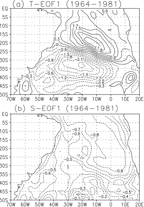
Fig. 3: Leading modes for the 1964-1981 period based on (a) T- EOF and (b) S-EOF, analysis respectively. Contour inter-val is (a) 0.3°C and (b) 0.1.

Leading SST patterns

The first three dominant SST patterns derived from the T-EOF analysis are displayed in Fig. 2, these patterns explain 19%, 10% and 8.5% of the variance re-spectively. T-EOF1 displays the typical north-south ori-ented dipole with dominant variability on interdecadal time scales. This pattern is recognized as the leading mode of SST variability in the South Atlantic and it is further discussed in the next section. T-EOF2 is charac-terized by a strong centre at around 20°W, 30°S and two centres of opposite-sign located south of Africa and along the South American coast, respectively. This is the only leading mode exhibiting a significant spectral peak on subannual time scales. These high-frequency SST vari-ability centres are located over the most energetic regions of oceanic meso-scale variability in the South Atlantic, the Brazil-Malvinas confluence and the Agulhas retro-flection (Chelton et al., 1990) . T-EOF3 exhibits an east-west dipole pattern at mid latitudes with significant vari-ability at interannual time scales. This mode presents a large correlation with ENSO, being highest when the ENSO index leads T-EOF3 by 6 months.

S-EOFs computed for the same time period and domain (not shown) were computed. Only the leading EOF mode agrees with the corresponding T-EOFs, S-EOF1 exhibits a dipole structure similar to T-S-EOF1 and it resembles the pattern found in other studies which also computed S-EOFs based on different datasets and time periods (Robertson et al., 2002 and references therein). The leading S-EOF shows variability in interdecadal and interannual time scales. This explains why to obtain the interdecadal signal in previous studies it was necessary to low-pass filter the SST anomalies (Venegas et al., 1997, Sterl and Hazeleger, 2002, among others).

Our results show that the EOF analysis performed in the time domain is useful to isolate the interdecadal variability, without filtering and also to determine lead-ing modes associated with independent spectral peaks.

The South Atlantic dipole

The dipolar structure that characterizes the lead-ing mode of SST variability in the South Atlantic is a very robust pattern. The VARIMAX rotation method was ap-plied to compute rotated EOFs based on both S-EOFs and T-EOFs and the dipole structure remained as the leading mode. To evaluate the existence of the dipole in the dataset for the pre-satellite period, a complementary study was carried out. We wish to determine the impact of the reduced data coverage in the mid-latitude South Atlantic on the dipole representation. The leading T-EOF for the period 1964-1981 shows the expected dipole struc-ture at interdecadal time scales although the spectral peak is found around 18 years (Fig. 3a). However, the leading S-EOF mode for the same period is characterized by a monopole pattern extending over the entire domain, with dominant interannual variability (Fig. 3b), while the interdecadal dipole pattern appears as the second

lead-ing mode. Venegas et al. (1997) obtained the same two first modes applying the S-EOF analysis to the COADS dataset. Moreover, Dommenget and Latif (2000) identi-fied a similar leading monopole pattern over the tropi-cal Atlantic. The existence of the South Atlantic monopole is questionable, as it seems to be influenced by the inho-mogeneous distribution of in-situ observations in the South Atlantic (Fig. 1). In contrast, the uneven data con-figuration does not appear to significantly affect the re-sults of the T-EOF analysis.

It is noticeable that the tropical action center of the South Atlantic dipole covers the region which some studies identified as the tropical South Atlantic mode (Dommenget and Latif, 2000 and references therein). Al-though a leading dipole pattern across the equator emerges from an S-EOF analysis performed over the tropical Atlantic, Mestas-Nuñez and Enfield (1999), Dommenget and Latif (2000), and others, have ques-tioned its existence and concluded that the centres of action across the equator present almost independent variability.

(15)

(a ) Tropic a l North Atla ntic

1 5 mo n th s 1 0 y e a r s

0 5 1 0 1 5 2 0 2 5 3 0 3 5 4 0 4 5 5 0

0 0 .0 5 0 .1 0 .1 5 0 .2 0 .2 5 0 .3

sp ec tr a l d en si ty ( ∫C 2/cpm)

(b) Tropic a l S outh Atla ntic

3 .5 y e a r s 1 4 y e a r s

0 5 1 0 1 5 2 0 2 5 3 0 3 5 4 0

0 0 .0 5 0 .1 0 .1 5 0 .2 0 .2 5 0 .3

sp ec tr a l de ns it y (∫ C 2/cpm)

(c ) Ex tra tropic a l S outh Atla ntic

14 y ears

10 months 0 5 10 15 20 25

0 0.05 0.1 0.15 0.2 0.25 0.3

fr e q u e n cy (cp m )

[image:15.595.66.266.84.481.2]

sp ec tr a l d en si ty ( ∫C 2/cpm)

Fig. 4: Spectra of the SST time series for (a) tropical North Atlantic center, (b) Tropical South Atlantic center and (c) Extratropical South Atlantic center. Expected red noise spec-tra (stippled) and 95% confidence lines are included.

Both the unrotated and rotated leading T-EOF resemble the dipole pattern across the equator with marginally significant variability on interdecadal time-scales.

In addition, for the period 1972-2000, we analysed the SST anomaly time-series in the three main centres of action found in the Atlantic basin. Two regions were se-lected in the South Atlantic (Fig. 1), which correspond to the tropical and extra-tropical centres found in T-EOF1 (Fig. 2). A third region was selected in the North Atlan-tic, over the centre of the tropical dipole. The latter is bounded by 35ºW-19ºW, 22ºN-15ºN (not shown).

The tropical North Atlantic variability exhibits a peak at around 10 years, which is close to the 95% confi-dence level. The South Atlantic regions show the maxi-mum variability at around 14 years. However, only the spectral amplitude for the extra-tropical region is sig-nificant at the 95% confidence level (Fig. 4).

While Dommenget and Latif (2000) have shown that SST anomalies at the two tropical centres are not significantly correlated, Sterl and Hazeleger (2002) found significant correlation between the SST anomalies of the two South Atlantic centres. In order to explore whether there is any frequency range for which SSTs in the three regions are significantly correlated, we computed the cross spectra, phase and coherence between each of the SST anomaly time series. The cross spectrum between the SST anomalies representing the South Atlantic di-pole shows a well-defined, significant peak at around 14 years. These observations suggest that the dipolar structure is a real physical mode of South Atlantic SST variability.

The SST cross spectrum for the cross-equatorial centres of action shows a marginally significant peak at around 14 years. Fig. 4 shows that although the tropical South Atlantic SSTs exhibits variability at around that period, the tropical North Atlantic SSTs do not. There-fore, in agreement with Mestas-Nuñez and Enfield (1999), Dommenget and Latif (2000), and references therein, the tropical Atlantic dipole does not appear to be a physical pattern of the SST variability at interannual time scales.

References

Chelton, D.B., M.G. Schlax, D.L. Witter, and J.G. Richman, 1990: Geosat altimeter observations of the surface circulation of the southern ocean. J. Geophys. Res., 95, 17877-17903. Dommenget, D., and M. Latif, 2000: Interannual to decadal variability in the Tropical Atlantic. J. Climate.,13, 777-792.

Kalnay, E., M. Kanamitsu, R. Kistler, W. Collins, D. Deaven, L. Gandin, M. Iredell, S. Saha, G. White, J. Woollen, Y. Zhu, A. Leetmaa, B. Reynolds, M. Chelliah, W. Ebisuzaki, W. Higgins, J. Janowiak, K.C. Mo, C. Ropelewski, J. Wang, Roy Jenne, and D. Joseph, 1996: The NCEP/NCAR 40-year reanalysis project. Bull. Amer. Meteor. Soc., 77, 437-471.

Hurrell, J.W., and K.E.Trenberth, 1999: Global sea surface tem-perature analyses: Multiple problems and their impli-cations for Climate Analysis, Modeling and Reanalysis. Bull. Amer. Meteor. Soc, 80, 2661-2678.

Mestas-Nuñez, A.M., and D.B. Enfield, 1999: Rotated global modes of non-ENSO sea surface temperature variabil-ity. J. Climate,12, 2734-2746.

Paegle, J.N., and K.C. Mo, 2002: Linkages between Summer Rainfall Variability over South America and Sea Sur-face Temperature Anomalies. J. Climate, 15, 1389–1407. Rayner, N.A., E.B. Horton, D.E. Parker, C.K. Folland, and R.B. Hackett, 1996: Version 2.2 of the Global Sea-Ice and Sea Surface Temperature Data Set, 1903-1994. Clim. Res. Tech. Note 74, Meteorological Office, Bracknell, UK., 21 pp. plus figures.

Reynolds, R.W., and T.M. Smith, 1994: Improved global sea sur-face temperature analysis using optimum interpolation. J. Climate, 7, 929-948.

(16)

Venegas, S.A., L.A. Mysak, and D.N. Straub, 1998: An interdecadal climate cycle in the South Atlantic and its links to other basins. J. Geophys. Res., 103, C11, 24723-24736.

Andrew W. Robertson1 and Carlos R. Mechoso2 1International Research Institute for Climate

Predic-tion, Palisades, NY, USA

2_{Dept. of Atmospheric Sciences, University of}

Cali-fornia, Los Angeles, CA, USA

1. Introduction

Hopes for seasonal-to-interannual climate predic-tion over South America are currently largely pinned on the influence of the Pacific and Atlantic Oceans on the atmospheric circulation over the continent. Here we fo-cus on the influence of the Atlantic anomalies on pre-cipitation during the austral summer when the South American Monsoon System (SAMS) is active.

SAMS precipitation variability can be divided roughly into two components: (1) a near-equatorial one associated with the Atlantic Intertropical Convergence Zone (ITCZ) and convection over Amazonia, and (2) a subtropical one associated with the South Atlantic Con-vergence Zone (SACZ) and related circulation features over the Pampas and SE South America. Each of these components involves a maritime atmospheric conver-gence zone together with continental convection, thus linking climate variability of the Atlantic Ocean with that over South America. This short article highlights selected aspects of the linkages between interannual climate vari-ability over the Atlantic and South America, and thus underscores the synergy between the climate pro-grammes centred on each one. Our emphasis is on societally important hydrological aspects: droughts and river flows.

2. Equatorial variability

The influence of equatorial Atlantic sea surface temperatures (SSTs) on droughts over NE Brazil is well documented (Hastenrath and Heller, 1977; Moura and Shukla, 1981; Mechoso and Lyons, 1988; Mechoso et al., 1990): droughts occur when the southward seasonal mi-gration of the ITCZ to its southernmost position in March–April is reduced due to anomalously warm (cold) SST anomalies over the tropical North (South) Atlantic, as well as to the direct Walker Cell-like influence of ENSO. The complex way in which ENSO interacts with the tropical Atlantic is not yet well understood. It has recently been proposed that the meridional gradient of SST between the tropical North Atlantic (TNA) and the

tropical South Atlantic (TSA) acts as a preconditioner on the direct ENSO impact on NE Brazil rainfall (Giannini et al., 2001). While most studies have focused on rainfall variability over NE Brazil, recent work suggests poten-tially useful one-year-ahead predictability of river flow in the Oros river, based on an empirical model with Niño-3, TSA and TNA SSTs as predictors (De Souza Filho and Lall, 2002).

The relationship between NE Brazil rainfall and the Atlantic Ocean appears rather confined to coastal regions, and a major challenge is to identify useful pre-dictable relationships between the broader-scale SAMS and the Atlantic. A major limitation to progress is the lack of long reliable records of precipitation. Riverflow records provide a valuable climate dataset, particularly for the Paraná-Paraguay rivers. These have their sources near 15o_{S and flow southward to the Plata estuary and} have reliable records since the early 1900s. As shown in Fig. 1, these records contain a statistically significant cy-cle at about 8 years (Robertson and Mechoso, 1998) whose period and phase closely match the near decadal cycle present in the North Atlantic Oscillation (NAO) (Robertson, 2001); each accounts for about 15% of the interannual variance. This covariability between the boreal winter NAO and the austral summer SAMS is intriguing. When SSTs are correlated with the 8-yr riverflow cycle, the typical NAO tripole signature in SST becomes clear (Fig. 2, page 35). The cold SST anomalies over the TNA that accompany enhanced river flows and a positive NAO suggest that an enhancement of the Links between the Atlantic Ocean and South American Climate Variability

Fig. 1: Leading oscillatory component of NAO (stippled, grey) and Paraná river (at Corrientes, black) timeseries, computed using Singular Spectrum Analysis (SSA) for each case with a window of 30 years. December–March averages.

1900 1920 1940 1960 1980 2000 4000.0

2000.0 0.0 2000.0 4000.0

Arbitrary Amplitude

Sterl, A., and W. Hazeleger, 2001: Patterns and wmechanisms of air-sea interaction in the South Atlantic Ocean. J. Cli-mate, submitted.

(17)

strength of the NE Trade winds over the tropical Atlan-tic may flux additional moisture into South America, which is then advected southward by the South Ameri-can low-level jet, another component of SAMS. The NCEP/NCAR reanalysis data does provide some sup-port for this conjecture (Nogues-Paegle et al., 2000), but the atmospheric record is too short and incomplete to distinguish this scenario from the alternatives, namely that a common forcing is simply reflected in both series or, indeed, that the Southern Hemisphere is forcing the North (Robertson et al., 2000).

3. Subtropical Variability

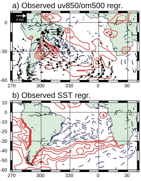
Variability of the SACZ dominates the atmos-pheric circulation over SE South America between about 20-40o_{S during austral summer. Most basically, the SACZ} exists in association with the southward transport of moisture from the tropics around the western margin of the subtropical anticyclone over the South Atlantic (Kodama, 1993). Fig. 3 (page 35) shows the leading interannual principal component of upper-tropospheric Reanalysis winds, regressed onto (a) 850-hPa winds and 500-hPa omega vertical velocity, and (b) SST. This lead-ing mode of circulation variability consists of an isolated Rossby wave with a dipole in the vertical motion field that reflects interannual changes in the intensity of the SACZ and “compensating” descent over the Pampas to the southwest (Robertson and Mechoso, 2000). Note that the low-level wind anomalies are such as to reinforce the vertical motion anomalies through low-level advection of heat and moisture.

This mode of variability is highly correlated with dipolar SST anomalies over the South Atlantic (Fig. 3b), with cold anomalies in the subtropics tending to accom-pany an intensified SACZ. Similar findings have been reported by Barros et al. (2000), while Diaz et al. (1998) have shown that interannual rainfall variability over Uruguay is correlated with a similar pattern of SST anomalies during austral summer. Since Uruguay lies under the southern pole of the omega dipole in Fig. 3a, dryer conditions are correlated with the SST pattern in Fig. 3b.

Fig. 3 does not show the SST-omega relationship that we would expect for subtropical SST anomalies forc-ing the accompanyforc-ing variations in the SACZ. One could argue that the SACZ variations are forcing variations in the SST below, with enhanced cloudiness leading to cold anomalies. However, the covariability with SST is com-plex, and surface fluxes of heat computed from the Reanalysis data do not show a coherent relationship.

Fig. 4 (page 36) shows the response of the UCLA atmospheric general circulation model to prescribing the SST anomaly in Fig. 3b. A statistically significant response is found in low-level circulation and precipitation. The GCM is able to capture the same broad circulation anomaly pattern seen in Fig. 3, but is of the opposite polarity to the observed one. This circulation pattern does

extend into the continent, although statistically signifi-cant rainfall anomalies are largely over the ocean. Quite similar findings are also reported by Barreiro et al. (2002) from an ensemble of long simulations with the CCM3 model. The implication of these GCM studies is that at-mospheric predictability associated SST anomalies over the subtropical South Atlantic is low.

4. Conclusions

The main linkages we have highlighted between the Atlantic Ocean and climate variability over South America, illustrated in Fig. 5 (page 36) are:

•

Changes in ITCZ position and intensity, affecting con-tinental convection through large-scale ascent and low-level moisture advection by the NE Trades. In-fluence of changes in cross-equatorial SST gradient, resulting from local and remote (ENSO, NAO) proc-esses. NAO influence seen at 8-yr period.

•

Changes in SACZ position and intensity, reflected in SST anomalies over the SW Atlantic. Large intrinsic interannual variability of the SACZ, modulated by ENSO, imprinted on Atlantic SST. Potential role for South Atlantic processes through changes in the strength and position of the subtropical anticyclone, or changes in ocean currents in the Brazil-Malvinas confluence region. Common spectral peak near 17 years.

An issue of concern for a better understanding of Atlantic-South American climatic linkages is the relative insensitivity of GCM-simulated rainfall anomalies over the continent that arise from interannual Atlantic SST anomalies. It is unclear to what extent this insensitivity is real, or whether it stems from inadequacies in the models over land.

5. References

Barreiro, M., P. Chang, and R. Saravanan, 2002: Variability of the South Atlantic Convergence zone simulated by an atmospheric general circulation model. J. Climate, 15, 745-763.

Barros V., M. Gonzalez, B. Liebmann, and I. Camilloni, 2000: Influence of the South Atlantic convergence zone and South Atlantic Sea surface temperature on interannual summer rainfall variability in Southeastern South America. Theor. Appl. Climatol., 67, 123-133.

Diaz, A.F., C.D. Studzinski, and C.R. Mechoso, 1998: Relation-ships between precipitation anomalies in Uruguay and Southern Brazil and sea surface temperatures in the Pacific and Atlantic oceans. J. Climate, 11, 251-271. De Souza Filho, F.A., and U. Lall, 2002: Seasonal to interannual

ensemble streamflow forecasts for Ceara, Brazil: Appli-cations of a multivariate semi-parametric algorithm. Water Resources Res., in press.

(18)

Hastenrath, S., and L. Heller, 1977: Dynamics of climate haz-ards in Northeast Brazil. Quart.J. Roy. Meteor. Soc., 103, 77-92.

Kodama, Y.-M., 1993: Large-scale common features of subtropi-cal precipitation zones (the Baiu frontal zone, the SPCZ, the SACZ) Part II: Conditions of the circulations for generating the STCZs. J. Meteor. Soc. Japan, 71, 581-610. Mechoso, C.R., and S.W. Lyons, 1988: On the atmospheric re-sponse to SST anomalies associated with the Atlantic warm event during 1984. J. Climate, 1, 422-428. Mechoso, C.R., S.W. Lyons, and J.A. Spahr, 1990: The impact of

sea surface temperature anomalies on the rainfall over northeast Brazil. J. Climate, 3, 812-826

Moura, A.D., and J. Shukla, 1981: On the dynamics of droughts in Northeast Brazil: Observations, theory and numeri-cal experiments with a general circulation model. J. Atmos. Sci., 38, 2653-2675.

Nogues-Paegle, J., A.W. Robertson, C.R. Mechoso, 2000: Rela-tionship between the North Atlantic Oscillation and river flow regimes of South America. Proc. 25th_Climate

Diagnostics and Prediction Workshop, Palisades, NY, 23-27 October, 2000, 323-326.

Robertson, A.W., 2001: On the influence of ocean-atmosphere interaction on the Arctic Oscillation in two general cir-culation models. J. Climate, 14, 3240-3254.

Robertson, A.W., and C.R. Mechoso, 1998: Interannual and decadal cycles in river flows of southeastern South America. J. Climate, 11, 2570-2581.

Robertson, A.W., and C.R. Mechoso, 2000: Interannual and interdecadal variability of the South Atlantic conver-gence zone. Mon. Wea. Rev., 128, 2947-2957.

Robertson, A.W., C.R. Mechoso, and Y.-J. Kim, 2000: The influ-ence of Atlantic sea surface tempearature on the North Atlantic Oscillation. J. Climate, 13, 122-138

Markus Jochum1, Paola Malanotte-Rizzoli1, Antonio

Busalacchi2_{, and Nelson Hogg}3

1_{Massachusetts Institute of Technology, Earth,}

Atmos-pheric and Planetary Sciences, Cambridge, MA, USA

2_{Earth System Science Interdisciplinary Center,}

University of Maryland, College Park, MD, USA

3_{Woods Hole Oceanographic Institution}

Woods Hole, MA, USA

corresponding e-mail: [email protected]

Introduction

Tropical Instability Waves (TIW) have first been observed by Legeckis (1977); they can been detected in the Pacific and Atlantic Oceans by their associated SST anomalies (see Fig. 1, page 36) and are generated in the equatorial mixed layer by shear instabilities of the equa-torial current system. Their period is between 20 and 40 days and their wavelength is of the order of 1000km (Legeckis (1977) and Weisberg and Weingartner (1988)). Hansen and Paul (1984) and Bryden and Brady (1989) show that the equatorward heat flux of the TIW exceeds the atmospheric heat flux at the equator. Thus, the posi-tion and strength of