Abstract— In this paper we analysis the subdiffusive structure of ISE 100 index price evaluation using the subordinated Ornstein-Uhlenbeck process. We use the subordinated Langevin equation approach to obtain a model of index prices. We use the inverse tempered stable distribution as a subordinator process. The subordinated Langevin equation approach is parallel to role played by Riemann-Liouville operator in fractional Fokker-Planck equation. Our aim to enhance the understanding of logarithmic asset returns behavior. We investigated the evolution of the subordinated Ornstein-Uhlenbeck process. The studied model combines the mean-reverting behavior, long range dependence and trapping events properties of index prices. To assess the capabilities of the model, we applied the model to the historical price data of the ISE100 index. The obtained results suggest that long range memory, trapping events, volatility clustering and fat tails and anomalous subdiffusive properties of interested index prices are captured by the proposed model.
Index Terms— Ornstein-Uhlenbeck Processes, Anomalous diffusion, Langevin equation, Subdiffusion.
I. INTRODUCTION
In 1900 Louis Bachelier proposed a Random Walk model to describe the fluctuations in financial market prices. Nowadays also the modeling of the financial price dynamics using stochastic processes has been an active research area in financial risk management, asset valuation and derivative pricing. In this study, we investigate time changed stochastic process models for financial time series. The one of the most important problems in financial modeling is to understand and appropriately model the price dynamics. The models of price process are the basis for the value of the contracts or assets under the uncertainty. Price process is given the complete description of uncertainly behavior of prices. Brownian motion is a continuous time model to describe diffusion of prices (particles) [1]. The diffusion processes are widely used for modeling real-world phenomena. The diffusion is the most prevalent form of the Physical transport. They are stochastic processes with continuous –time and continuous-space. In application, the diffusion processes are important tools in Physic, Biology and Finance etc. A general diffusion process is given by
t
t
tt X dt X dB
dX ; ; . As a special case
Xt
Xt ; and
Xt;
Xt and it was used to model the spot price of a stock by Black-Scholes option pricingÖ.Önalan is with the Faculty of Business Administration, Marmara University, Bahçelievler, Istanbul, Turkey
(e-mail: [email protected]).
formula. All these models based on Brownian motion have normal distribution. That assumption is not consistent with empirical properties as heavy tailed and skewed marginal distributions, trapping events, non independence. The anomalous diffusive behaviors were observed a variety of Physical, Biological and Financial systems [19]. (Magdziarz,M and Gajda,J(2012)) proposed the geometric Brownian motion time- changed by infinitely divisible inverse subordinators to reflect underlying anomalous diffusive behavior [23].
The anomalous diffusion (subdiffusion) usually described using (Fractional) Fokker-Planck equation which describes probability density function of the diffusion (sub diffusion) and derived from continuous-time random walk with heavy tailed waiting times. The main idea in generalization of the Ornstein-Uhlenbeck process is to replacement another stochastic process.
The continuous time models are rather popular in finance. The Classic Ornstein-Uhlenbeck process (OU) is one of the basic continuous time models. It is a univariate continuous time Markov process and has a bounded variance and has a stationary probability density function. Vasicek(1977) [2] used the Ornstein-Uhlenbeck (OU) process to model the spot interest rate. Non-Gaussian OU processes are an important special case of Markov processes with jumps [15].
The description of waiting time which corresponding to trapping events is an important in the analysis of time changed processes[1]. Generally the subdiffusion is described by fractional Fokker-Planck equation which is derived from the power law waiting times. The solution of Fokker-Planck-type equation is equal to the probability density function of the subordinated process X
S
t
[22].The Ornstein-Uhlenbeck process denotes the mean-reverting property which means that if process is above the long run mean, then drift become negative then process be pulled to mean level. Likewise if process is below the long range mean level then process is pulled again to long run mean level. The spread of a sub diffusive random variable (asset price or particle) is slowed compared Brownian motion predicts. To modeling the kind of diffusion, the time structure of process is changed. The time changed process has not Markovian Dynamics. The idea of time-change of process was introduced by Bochner,S.(1949)[24]. It can be consider the replacement of real time in the consider process (it call external process) by some subordinator (non decreasing process with stationary, independent increments).The inverse subordinator is used a new random operational time for external process [8].
In this study, we consider Ornstein-Uhlenbeck process as
Subdiffusive Ornstein-Uhlenbeck Processes and
Applications to Finance
external process and as a subordinator inverse tempered stable distribution (the first passage time). We change the time of base process with this inverse subordinator. The trajectory of subordinator has increments of length
random time moments and it is driven by tempered stable distribution. We use the subordinator process as the operational time. We use the tempered stable distribution to model the waiting times (motionless periods). It leads a subdiffusive behaviour in short times and diffusive behaviour in longer times. In this study we will use Langevin approach to analyze the subdiffusive behavior.
The paper is organized as follows. In section 2, we review some basic facts of the Langevin equation and Ornstein-Uhlenbeck process and its parameter estimation problem. In section 3, we give subdiffusion concept then we describe the subordinated Ornstein-Uhlenbeck processes with inverse tempered stable subordinator. In section 4, we apply the examined models to daily ISE100 index data, section 5 provides the conclusions.
II. THE ORNSTEIN-UHLENBECK PROCESSES
A. Langevin Equation
The Langevin equation describes the main characteristics of a general random motion in the random environments. This equation was produced by Langevin(1908) [25] and become one of the most fundamental stochastic differential equation especially in Physics[26]. The Langevin approach assumes that the particle moves in the fluid medium follows Newtonian mechanic under the influence of external force and friction. The influence of the molecules of the surrounding medium are modelled a random noise term. This equation also has applications in Biology, Physical Chemistry and Engineering. Let we consider a particle of mass m moves along a line is subject to two forces. We will assume that the deterministic external force F is zero. A fractional force that is proportional to particle velocity and a random white noise force that it models random fluctuations. Let Vt denotes the velocity of the particle which a Brownian motion of a free point particle in a fluid at time t. One dimensional Langevin equation is given by
t t t
V dt dV
m (1) Where mis the particle’s mass,Vtis the friction force,
is the friction coefficient , is strength of the noise, t is the random force. Dividing the equation by
m
t t
t V
dt
dV
(2) Where m0 and m are constant [5]. We can use dBt dt instead oft. We write the above equation in differential form as
t t
t Vdt dB
dV (3) Where V0v0 is fixed deterministic quantity. The process
t
B is standard Brownian motion.
B. Ornstein-Uhlenbeck Processes
The classic Ornstein-Uhlenbeck process (OU) was proposed in 1930 by G.E. Uhlenbeck and L.S. Ornstein [27]. Essentially, the model (OU) proposed to describe velocity of
Brownian particle immersed in a fluid. It is unique continuous time Markov process possessing a stationary distribution. The Ornstein-Uhlenbeck processes driven by Lévy processes are a special case of Markov processes with jumps [28].
The process Vt satisfies the Langevin equation by equation (3) is called Ornstein-Uhlenbeck process.
t
s s t t
t v e e ds
V
0
0 (4)
The Vasicek model assumes that instantaneous short rate
xt Vt
follows an OU process with constant coefficients,,,
, 0 t t
t x dt dB
dx (5) The explicit solution to the above SDE between any two instants
s
andt
, with 0st can be easily obtained from the solution to the Ornstein-Uhlenbeck SDE, namely:
t
s u u t s
t s s t
t e x e e e dB
x 1 (6)
Where: long term mean, :the velocity of the process to.The conditional mean and conditional variance of xst given xsis described as follows
t s ss
t x x e
x
E (7)
t s
stx e
x
Var
2 2
1
2 (8) If the time increases the mean tent to the long term value and variance remains bounded, this implies mean-reverting process. The covariance of the process at two different times
t and tsgiven by
1
, , 02
, 2
2
e e t s
x x
Cov t t s t s
(9) Conditional distribution of xst given xs is
ts ts
s e e
x
N
2 1 2
2
, (10) When,t the distribution of the Ornstein-Uhlenbeck process is stationary and Gaussian with mean and standard deviation 2 2 .The transition density function of the above Ornstein-Uhlenbeck process is given by
22
2 0
2 exp 2
1 ,
t t
t
x x
t x p
(11) Above OU process
xt t0 also can be denote by a time scaled Brownian motion,
t
t
tt
t x e e Be e
x
1
2
1 2
0 (12)
The time and space are shrinking; self-similar Brownian motion can be transformed into the stationary Ornstein-Uhlenbeck process [29]. The process
xt t0 can be discrete using Euler Scheme with time stepttiti1,
t
tt t
t x x t tZ
T t
the number of observations. We assume that we observed the process at discrete time points. Discrete time observations was denoted by X
x0,x1,...xn
then Ornstein-Uhlenbeck process is given by
it t
t i t t
i Z
e e
x e x
2 1 1
2
1
(14) whereZi~N
0,1 and i1,2,...,n .C. Parameter Estimation of Ornstein-Uhlenbeck Process
Maximum Likelihood Method: The conditional PDF of rate i
x given the xi1 (for brevity x
ti is denoted byxi) given by
2
2 1 2
1
2 exp
2 1
e x x x
x
f i i i i (15)
(for details look[30]).
n
t
n
t t n
t t t t n
t
n
t t
t x n x x x x
x n
1 1 1
1 1 1
2
1 1 2
1 ln
ln ˆ
(16)
n
t
t t x e x n
e 1
ˆ 1 ˆ
1
1 1
ˆ
(17)
n
t
t
t x e
x n
e 1
2 ˆ 1 ˆ
2
2 1 ˆ ˆ
1 ˆ 2
ˆ
(18)
OLS Method : We can write the value of random variable
x
at timet
conditional onx
t1 as follows
s t
t s t t
t t
t e x e e dW
x
1 1
1
If we take the time increments t1 and we consider AR(1) model as xt cbxt1t comparing above equation and AR(1) model we have that,
e
c 1 , be and
1e2
2. Finally we obtain the OLS estimators as,
bˆ ln ˆ ,
b c
ˆ 1
ˆ ˆ
and
bˆ 1 2lnbˆ ˆ ˆ2
Where ˆ is standard deviation of residuals of regression equation thextcˆbˆxt1et.
III. SUBDIFFUSIVE MOTION
The idea of subordination firstly was introduced by Bohner(1949). It is based on the replacement of real time in the external process by a subordinator which plays the role of random operational time [8]. The means of subordination of processX
with another process S
t is to randomize the physical time t byS
t , then we obtain a new subordinated process asY
t X
S
t
. It is a continuous time random walk (CTRW).We can consider the diffusion of a price (particle) as a sequence of independent random jumps occurring instantaneously. Other words, the waiting time between the successive jumps and jump length are random variables. So the subordinated process
t X
S
t
Y is combination of two independent processes. One of them is a parent process
X
. It is also called the external process. The second oneS
t is the waiting timeprocess. It describes the new operational time S
t of the system [31]. The inverse subordinator is described by following first passage time relation,
t
T
t
S inf0: (19) where
T
is the strictly increasing Levy process. It is a pure-jump process. For every jump of T
, there is a corresponding flat period of its inverse
S
t
.The flat periods of
S
t
represent the waiting time which the subdiffusion process gets immobilized in the trap. If the jumps have normal distribution and waiting times with exponential distribution, this case leads to the normal diffusion, if the jump lengthiest have normal distribution and the waiting times have a power-law distribution this leads to anomalous model. A non-negative random variable Tis called infinitely divisible distribution, if its Laplace transform takes the following form,E
euT
e u (20) Ifg
t, is the PDF of T
then Its Laplace transform is defined by
uT
ut
ue dt t g e e
E
0
, (21) where
. is called Laplace exponent and defined by
0
1 e vdx u
u ux
whereis drift parameter and v
dx is a Lévy measure[32]. For a stochastic process with an infinitely divisible distribution, the function
u should be nonnegative and completely monotone recording to first derivative and
0 0. If we choice the Laplace exponent as
u u , then we obtain a tempered stable subordinator.
A. Subordinators
One of the most popular statistical models of anomalous diffusion is the continuous time random walk model (CTRW) which corresponds to the fractional diffusion equation driven by Lévy diffusion process. In a CTRW model, the each step is characterized by corresponding waiting time and the displacement in space.
The process driven by inverse subordinators are strongly related to the continuous time random walk. The distribution of the subordinator increments corresponding to observed constant time periods (motionless periods). In applications, we can choice the different subordinators. These subordinators belong to the infinitely divisible distributions class. If we choice the Laplace exponent of subordinator is a power law i.e.
u u then we obtain a pure anomalous subdiffusive process. [12]. Subordinators are sum of i.i.d. random variables with an infinitely divisible PDF. The examples of them, Gaussian, inverse Gaussian, stable, tempered stable, exponential, gamma, compound Poisson, Pareto, Linnik and Mittag-Leffler. The non-negative infinitely divisible random variables are fully characterized by the exponentially weighted function. If
t,
tS can be represent by
t g
s ds f t
, ,The Laplace transform of f
,t with respect to t is obtained as follows [32],
e u uu u
f , ~
(22) Generally a subordinator whose Laplace exponent is the power law leads to a model of the pure anomalous diffusion and their MSD grows as a power law in time. For example if
t BtY is a standard Brownian motion then for
u u the subordinated process B
S
t
is proportional to
1
t as t0 and proportional to t as t. Hence the process B
S
t
occupies an intermediate place between pure subdiffusion which the second moment grows like t and normal diffusion where the second moment is proportional tot
.B
is Brownian motion is 12 -self-similar so, B
12B
1d
, T
stable Levy motion is the 1 self-similar so, T
1T
1d
and inverse
subordinator S
t
t T
t
d . We can obtain subordinated
process as follows[32].
t B
S
t
S
t
12B1 t 2
T
1
2B
1Y d
(23)
1) The Mittag-Leffler Distribution as a Subordinator
Mittag-Leffler distribution is an example of power law distributed waiting times. The generalized Mittag-Leffler function is defined by
0 , n n n z zE
Let
X
be a Mittag-Leffler random variable the PDF ofX
on
0, has the Laplace transform
s
1s
1 where s0,01 and 0. To obtain Mittag-Leffler random number we use the Kuzubowski and Rachev simulation technique [33],
1 cos tan sin log V UT (24)
where U,V
0,1 are uniform random variables and T is a Mittag-Leffler random number as a second approach we can use following classic method1 , 1 1
T U
T where U,1 is a skew Levy stable random variable and T1logU 8.
2) Tempered Stable Subordinator
The tempered stable distribution which is extension of stable distribution is obtained by multiplying an exponential tempering function of probability density function stable distribution. We consider the skew tempered stable random variable
T
.The probability density functions (PDFs) of skew tempered stable distributions are given by
1 , log 1 1 , 1 1 x p e x p e x p U x U xT (25)
where pT
. is the PDF of the tempered stable randomvariable T and pU
. is a PDF of random variable U with the stable distribution with index of stability, skewness1
, mean 0 and scale parameter
1 2 cos for 1
, 2 for 1[34].
4 2 2 3 3 2 4 2 2 3 3 2 3 2 3 6 ˆ m m m m m m m m ,
3 2 ˆ 2ˆ
m
m
(26)
Where 1
, 2,3,41
k E E n m n i k ik and Eis a sample mean
of motionless periods of prices. In application the parameters in tempered stable distributions can be estimated by the real market data. We will simulate operational time inverse tempered stable subordinator S
t as the step size T N and
tii:i1,2,...,N
[34], [35].
min
kN:T
k ti
1
.S (27) where 01 and
T
0 denotes a strictly increasing a
stable Levy motion with tempered stable waiting times between successive jumps. 0 Tempering parameter is and 01 is stability index.
a) Generate exponential random variable
E
with mean
1. b) T
k T
k1
Zk, T
0 0,k1,2,...N
1 11 cos 2
. cos 2 sin W V V V V Zk
where V is uniformly distributed on
2, 2
and Wexponentially distributed with mean 1.)
c
If EkZk put T
k S
k , k1,2,...N otherwise go to step (a).B. The Mean Squared Displacement (MSD)
In the study of diffusion processes, statistical quantification of temporal dispersion of diffusions is an important issue. To that and we use the mean squared displacement (MSD). In the anomalous diffusion case, the variance in the position of particle scales other than linearly with time. The MSD behaves like power function i.e.,
x
t2 x
t
2 ~t. The value of parameter characterizes the stochastic properties of the observed process. We can calculate the MSD values for different values as,
2 t x t xMSD
n x x x x x xMSD n n
2 1 2 1 2 2 0 1 ...
1
1 ... 2 2 2 2 1 3 2 0 2 n x x x x x xMSD n n
2 ... 3 2 3 2 1 4 2 0 3 n x x x x x xMSD n n
For varying time lagstnnt, MSD is calculated as follows,
1 1 2 1 1 2 11 N n
i
i n i
n x x
n N t x
T xt xt dt
T T MSD
0
2
1 ,
Where is the lag time i.e., a fixed time window and T is the total time. If there are strong difference between the moving time averages and ensemble average it implies the non ergodicity such systems. The parametercan be obtained by measuring the slope of the logarithm of the MSD as dependent on the logarithm on time. The asymptotically MSD
,T ~1 can be observed. Finally we can consider following approach for MSD,
n
k
k k k k k
k t t M t
X E
1
1 2
1 2
where0t0t1...tnt and variable order function.
t 1t100,
0t100
Which represent that a
decelerating diffusion process, shift from normal to sub diffusion for M1,1 we obtain the corresponding MSD-time curves. We calculate the MSD for the sample
x1,x2,...,xN
with stationary increments as follows
Nk
k k
N x x N
N M
1
2
1 ,.. 2 , 1 , 1
The MDS is a function of and it is a random variable. The MSD behaves likeMN
~. For 01 the process is subdiffusive. This type behaviour usually observed disordered systems. A subdiffusive process has long memory properties. Subdiffusive systems usually described Levy type statistics and heavy tailed distributions, if 1 the observed process represent the super diffusive behaviour. This case usually observed the system unstable or in transient state and if 1 the observed process denotes the normal diffusion so systems randomly fluctuation [3]. If the sample comes from a Hself similar Levy stable process with stationary increments then largeN k, sample MSD asymptotically behaviour as a power law MN
k ~k2d1, dH1, estimating the parameter2d1, we obtain information about the diffusive characteristics of the real process. When0 1
H
d then the process is sub diffusive when 0
1
H
d the process is super diffusive [8].
IV. THE SUBDIFFUSIVE ORNSTEIN-UHLENBECK PROCESS
In this section, we describe the time changed a OU process
t X
S
t
Y .We choice the inverse tempered alpha stable distribution as a subordinator process, to simulate the price series, we used the following model which is proposed by L.Longjin., et al.(2012) [14].
t
k
t
k k tt Y FY t DY t Z
Y 1 1, 1 2 1, 112 12 (27)
whereZk~N
0,1, kS
k S
k1
. We will use
xt x tF , 0.0116 and D
x,t 0.6x14tV. APPLICATIONS TO REAL DATA
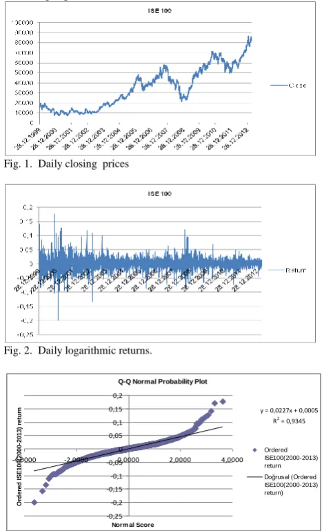
In this section the capabilities of the considered model are tested on ISE100 index return data. We use the subordinated Ornstein-Uhlenbeck process to model ISE100 index closing price behaviour. Historical prices data of ISE 100 index chosen from 04.01.2000 to 04.01.2013 and 3303 daily
observations. We obtained the data from Yahoo finance web page. The empirical log returns xt at time t0of the prices
tS over a period t0 are defined by
t t
S
tS
[image:5.595.306.540.170.555.2]xtln ln . For we will use the daily returns, we set t1252 (data collected once a day). In order to characterize the probabilistic structure of the price process, we give the basic descriptive plots for the daily closing prices and returns for ISE100 index is presented in the following figures.
Fig. 1. Daily closing prices
Fig. 2. Daily logarithmic returns.
Q-Q Normal Probability Plot
y = 0,0227x + 0,0005 R2 = 0,9345
-0,25 -0,2 -0,15 -0,1 -0,05 0 0,05 0,1 0,15 0,2
-4,0000 -2,0000 0,0000 2,0000 4,0000
Norm al Score
O
rd
e
re
d
I
S
E
1
0
0
(2
0
0
0
-2
0
1
3
)
re
tu
rn
Ordered ISE100(2000-2013) return
Doğrusal (Ordered ISE100(2000-2013) return)
Fig. 3. Empirical and standard normal quantiles
The price and log return paths denotes the long memory and mean-reverting behavior of series. We did not observe any trend at data. The figure2 illustrates that large moves follow large moves up and down and small moves follow small moves so there is volatility clustering for index returns. Q-Q plots indicate the S-shape curves this denotes the non normal returns in time series. Furthermore return series has heavy tails. These empirical distributions confirm the non normal distribution for ISE 100 index returns. We give the descriptive statistics in the following table1 for the ISE100 index returns.
TABLEI
SUMMARY STATISTICS OF DAILY RETURN FOR ISE 100 INDEX
Index Mean Std.dev Min Max Skew
S
Kurt K
KS Stat. ISE10
0
0,000 5
0,024 -0,2 0,178 0,025 6,944 0,07
normal distribution is zero. The index has positive skewness. This denotes that return distribution is not symmetric. The distribution has a long right tail. The easy way to quantify the distribution of log returns. The value of Kurt3 indicates a heavy tail. Empirical kurtosis value exceeds value of three. So the distribution is leptokurtic relative to normal distribution. This means that the distribution has heavy tails.
To investigate the dependence structure on the observed time series we calculate and plot empirical autocorrelation function (ACF)
k given for a set of the observationsn x x
x1, 2,..., .
k n
i
k i
i x x x
x n k
1
1
Where, n is the number of observations in sample and k is the lag.
Autocorrelation(ISE100 index return)
-0,2 0 0,2 0,4 0,6 0,8 1 1,2
0 2 4 6 8 10 12 14 16
Lags
[image:6.595.307.554.133.387.2]ACF Seri 1
Fig. 4. Autocorrelation function of ISE100 index returns.
We will apply the autocorrelation test to check to the independence of the time series. The autocorrelation values are near to the zero so we can say that examined time series is independent. Before thinking about fitting a specific mean reverting process to available data, we have to check the validity of the mean reversion assumption. Simple way to do this is to test for stationary. Let xt represent the log-price.
t t t b bx x
0 1 1 , t~N
0,1The testing the mean reversion in a sample time series of returns is to check whether in the above equation the coefficient b1 is significantly different from 1. This means
that xt can be considered as a stationary process. If b1 1 the process is explosive and it will be never revert back to long-range value, if b1 1 the process is a unit-root process and if 1b10 the process is a mean reverting. Time interval between the observations t1n.Furthermore we should be performed to check whether the coefficient
b
1 is negative. Test statistics is given by 2 1
1 2
1 ˆ ˆ
ˆ
n
i i
test b x x
t
where n is number of sample points and
2 1
1
2
2 ˆ
2 1
ˆ
n
i
i
i x
x n
, If ttest 2 then the result is significant. Using the linear regression we obtained
491285 . 0
H . This means that an increas will tent to be followed by a decreas or a decreas will be followed by an increas.This behavior is sometimes called mean reversion.The strength of this mean reversion increases as Happroaches 0[18]. As a result observed time series has mean reverting property. For an arbitrary time lag , MSD of fractional Brownian motion satisfies, that relation
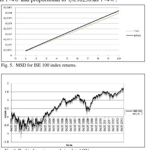
H [image:6.595.50.284.246.349.2]MSD ~2 . This result represent that ISE100 index price series has subdiffusive dynamics. We know that2H0,982569. On the other hand MSD
t t0.982569 for ISE100 index prices. The MSD of the subordinated process X
S
t
is proportional to t0.982569
10.0,982569
as t0 and proportional to t 0.982569as t.Fig. 5. MSD for ISE 100 index returns.
Fig. 6. Real index returns and simulated OU process.
Let be observed time seriesX
x1,x2,...,xn
. To analyze time changed the index return; we decompose the observed series into two X1 and X2vectors. The elements of thevector
1
,..., ,2 1 1 l l ln
X are lengths of constant periods of X .
The other vector
2
,..., , 2 1
2 m m mn
X is obtained from the values of X corresponding to the non-constant periods. We assume that the immobile periods of process X are equal to the jumps of the process T
t [34].Fig. 7. The distribution of the constant periods(trapping events)
We assume that the vector X1 consist of iid random
variable from the tempered stable distribution.
[image:6.595.307.552.516.638.2] [image:6.595.307.552.670.773.2]Fig.9. Subdiffusive Ornstein-Uhlenbeck model for ISE100 index returns
TABLEII
THE ESTIMATION OF PARAMETER FORVECTORX1
Index estimation
ISE 100 0.68988
TABLEIII
THEMODEL PARAMETER ESTIMATION FOR ISE100 INDEX RETURNS
Index aˆ bˆ ˆ ˆ ˆ
ISE100 0.00051 0.0121 483.54 0.000526 0.7342
VI. CONCLUSIONS
In this paper, we investigated the time changed Ornstein-Uhlenbeck process with application to index returns. As a subordinator we used inverse stable tempered distribution and shortly revisited some alternative subordinators. We presented the estimation methods for unknown parameters in this process. Motivation to choice for tempered stable distribution based on the empirical properties of index return data. The results represent that the proposed model can be capture the stylized facts which is observed return time series and trapping events. The pricing of assets, the hedging of contingent claims, the valuation of investments and risk management heavily based on the stochastic model which is describe the behavior of considered the real process. As a consequence, the changing the time of the model with a suitable subordinator can be useful approach to improve the financial returns modeling.
REFERENCES
[1] J.Janczura and A.Wylomanska,”Anomalous diffusion models: different type of subordinator distributions”, Acta Physica Polonica B, vol.43, n0.5, 2012, pp.1001-1016.
[2] O.Vasicek,"An equilibrium characterization of the term structure", J.Financial Economics 5, 1977,pp. 177–188.
[3] A.Szczurek,,et.al.,”Dynamics of carbon dioxide concentration in door air”, Stoch. Environ. Res. Risk., 2014. .
[4] I.I.Elizar,and M.F.,Shlesinger,” Langevin unification of fractional motions”, J.Phys.A: Math. Theor., 2012, 45,pp.162002.
[5] J.Hunter, Lecture notes on Applied Mathematics: Methods and Models, Department of Mathematics, University of California, Davis. 2009, ch.5.
[6] J.P.Bouchaud and R.Cont,”A Langevin approach to stock market fluctuations and crashes”, Eur. Phys. J.B ,1998,6, no.4, pp.543-550. [7] G.E.Uhlenbeck and L.Ornstein,”On the theory of Brownian motion”,
Phys. Rev. 36, 1930,pp. 823–841.
[8] M.Teuerle, A.Wylomanska and G.Sikora, “Modeling anomalous diffusion by a subordinated fractional Levy-Stable process”, Journal of Statistical Mechanics: Theory and Experiment, 2013,pp. P05016. [9] Q.X.Sun and W.Xiao,” An empirical estimation for mean-reverting
coal prices with long memory”, Economic Modeling 33, 2013, pp.174-181.
[10] K.Burnecki, M.Magdziarz, A.Weron,” Identification and Validation of Fractional Subdiffusion Dynamics”, In Fractional Dynamics, 2011, Chapter 14, p.133.
[11] A.Kaeck and C.Alexander,” Continuous-time VIX Dynamics: On the role of stochastic volatility of volatility”, International Review of Financial Analysis, 2013, ,pp.28,46-56.
[12] M.Magsziarz, J.Gajda,”Anomalous dynamics of Black-Scholes model time changed by inverse subordinators”,Acta Physica Polonica B, vol.43, no.5,2012, pp.1093-1109.
[13] M.Magdziarz,” Black-Scholes formula in Subdiffusive regime”, J. Stat. Phys. 136,2009, pp.553-564.
[14] L.Longjin, Q.Weiyuan, and R.,Fuyao,” Fractional Fokker-Planck equation with space and time dependent drift and diffusion”, J. Stat. Phys. 149,, 2012, pp.619-628.
[15] Z.Shibin and Z.Xinsheng,”Exact simulation of IG-OU processes”, Methodol Comput Appl Probab10, 2008, pp.337-355.
[16] J.Janczura et.at,”Stochastic modeling of indoor air temperature”. Stat. Phys. 2013,DOI 10.1007/s10955-013-0794-9.
[17] I.M.Sokolov,”Models of anomalous diffusion in crowded environments” ,The Royal Society of Chemistry, Soft Matter8, 2012, pp.9043-9052.
[18] J.Golder, M.Joelson,,M.C..,Neel,.,Di L.Pietro,”A time fractional model to represent rainfall process”,Water Science and Engineering,7(1), 2014, pp.32-40.
[19] J.Janczura, S.Orzel and AWylomanska,”Subordinated -stable Ornstein- Uhlenbeck process as a tool for financial data description”, Physica A,390, 2011, pp.4379-4387.
[20] K.C.Chan, G.A.Karolyi, F.A.Longstaf and A.B.Sanders, ”An empirical investigation of alternative models of the short-term interest rate”, Journal of Finance, 47, 1992,pp.1209-1227,
[21] J.Obchowski, A.Wylomanska,”Ornstein-Uhlenbeck process with non-Gaussian structure”,Acta Physica Polonica B, vol.44, no.5, 2013, pp.1123-1135.
[22] Li, Guo-Hua, H.Zhang and L.Muo-Kang,,”A multidimensional subdiffusion model: An arbitrage free market”, Chin. Phys. B, vol.21, no.12,2012, pp.128901-1-128901-7.
[23] M.Magdziarz and J.Gajda,”Anomalous Dynamics of Black-Scholes model time-changed by inverse subordinators”, Acta Physica Polonica B, vol.43, no.5,2012, pp.1093-1109.
[24] S.Bochner, Proc. Natl. Acad.Sci,35,1949, pp.368.
[25] P. Langevin, "Sur la théorie de mouvement Brownien" C.R. Acad. Sci. Paris , 146 ,1908, pp. 530–533.
[26] I.I.Eliazar and,M.F.Shlesinger,”Langevin unification of fractional motion”, J.Phys.A:Math.Theor.45, 2012, pp.162002.
[27] G.E. Uhlenbeck and L.S. Ornstein, "On the theory of Brownian motion" Phys. Rev. , 36 (1930) pp. 823–841
[28] Z.ShiBin and Z.X, Sheng, ”Test for autocorrelation change in discretely observed Ornstein-Uhlenbeck processes driven by Levy processes”, Sci.Cina Math.vol.56. no.2,2013.
[29] M.Magdziarz andA.Weron,”Ergodic properties of anomalous diffusion processes”,Annals of Physics 326, 2011,,pp.2431-2445 [30] A.Zoglat et al.,”A mean-reverting model of the short term interbank
interest rate: the Moroccan case”, Journal of Finance and Investment Analysis, vol.2, no.3,2013,pp.55-67.
[31] A.Stanislawsky, K.Weron, and A.Weron, ”Anomalous diffusion with transient subordinators: A link to compound relaxion laws”, The journal of Chemical Physics 140, 2014, pp.054113.
[32] J.Gajda and A.Wyłomańska,"Fokker–Planck type equations associated with fractional Brownian motion controlled by infinitely divisible processes", Physica A 405, 2014,pp. 104–113.
[33] D.Fulger, E.Scalas and G.Germano,”Monte Carlo simulation of uncoupled continuous-time random walks yielding a stochastic solution of the spaces-time fractional diffusion equation”, Phys.Rev.E,77,2008,pp.1-7.
[34] J.Gajda and A.Wyłomańska,"Tempered stable Lévy motion driven by stable subordinator", Physica A 392, 2013, pp. 3168–3176.