How well does active learning actually work? Time based evaluation of cost reduction strategies for language documentation

How well does active learning

actually

work? Time-based evaluation of

cost-reduction strategies for language documentation.

Jason Baldridge

Department of Linguistics The University of Texas at Austin

[email protected]

Alexis Palmer

Computational Linguistics Saarland University

[email protected]

Abstract

Machine involvement has the potential to speed up language documentation. We as-sess this potential with timed annotation experiments that consider annotator exper-tise, example selection methods, and sug-gestions from a machine classifier. We find that better example selection and la-bel suggestions improve efficiency, but ef-fectiveness depends strongly on annota-tor expertise. Our expert performed best with uncertainty selection, but gained lit-tle from suggestions. Our non-expert per-formed best with random selection and suggestions. The results underscore the importance both of measuring annotation cost reductions with respect to time and of the need for cost-sensitive learning meth-ods that adapt to annotators.

1 Introduction

Data annotated with linguistically interesting la-bels is used in a wide variety of contexts. Com-putational linguists generally use annotated data as training and evaluation material for natural lan-guage processing systems; corpus linguists use it to test hypotheses about language; documentary linguists create interlinear glossed texts to pre-serve examples of endangered languages and hy-potheses about the grammars of those languages. Regardless of the context, creating annotated data is costly in terms of time and/or money. Since both time and money are undeniably in limited supply, there is a widely shared desire to reduce this cost.

Reducing cost involves strategies that do more with fewer human-annotated labels and/or reduce the per-label cost. An example of the former is ac-tive learning, which focuses annotation effort on data points selected by the learner(s) for their ex-pected utility in developing a more accurate model

(Settles, 2009). Examples of the latter include providing suggestions from a machine labeler and using extremely cheap human labelers, e.g. with the Amazon Mechanical Turk (Snow et al., 2008). Different techniques may be more or less appli-cable depending on the language being annotated, the kind of labels which are desired (tags, syntac-tic structures, etc.), and the desired use of the an-notated data (e.g., for training models, testing lin-guistic hypotheses, or preserving a language).

This paper discusses experiments that measure the effectiveness of machine-aided annotation for language documentation using both active learn-ing simulation experiments and annotation ex-periments which involve actual documentary lin-guists interacting with machine example selec-tion and label suggesselec-tion. Specifically, we deal with the task of labeling morphemes of the Mayan language Uspanteko with fine-grained parts-of-speech. We also run active learning simulation experiments for part-of-speech tagging for Dan-ish, Dutch, EnglDan-ish, SwedDan-ish, and Uspanteko to show the validity of our models and methods in a standard setting. For Uspanteko, we provide re-sults from annotation experiments in which anno-tation cost is measured in terms of the actual an-notation time required while varying three factors: (1) example selection, (2) machine label sugges-tions, and (3) annotator expertise.

Our findings indicate that there is consider-able promise for reducing the cost of produc-ing IGT, but they also demonstrate considerable variation due to the interaction of these factors. This suggests different prescriptions for appropri-ate strappropri-ategies in different contexts. Most clearly, the worst performing strategy—by far—is that used in nearly all documentary work: sequential annotation without automation. Also, our expert annotator did best with examples picked by un-certainty selection, while our non-expert did best with random selection aided by machine label

Language #words-tr #words-dev #tags #sents-tr #sents-dev Avg.sent Avg.tr.sent Avg.dev.sent

Danish 62825 31561 10 3570 1618 18.18 17.60 19.50

Dutch 129586 65483 13 9365 3982 14.61 13.84 16.44

English 167593 131768 45 6945 5527 24.00 24.13 23.84

Swedish 127684 63783 41 7326 3714 17.34 17.43 17.17

Uspanteko 43473 19906 69 7423 3288 5.92 5.86 6.05

Table 1: Corpora: number of words and sentences, number of possible tags, and average sentence length.

gestions. This difference confirms the importance of cost-sensitive active learning strategies that are not just learner-guided, but also take into account modeling of the annotators (Settles et al., 2008; Haertel et al., 2008; Vijayanarasimhan and Grau-man, 2008). Finally, we confirm the importance of using actual annotation time to measure annota-tion cost: a unit-cost assumpannota-tion—even at a fine-grained level—can dramatically misrepresent the actual effectiveness of different strategies.

2 Task and data

Annotation task: language documentation The amount of money spent on obtaining human annotations is an extremely important concern in much language annotation. However, there is a further urgency for annotation in the case of lan-guage documentation: lanlan-guages are dying at the rate of two each month. By the end of this cen-tury, half of the approximately 6000 extant spoken languages will cease to be transmitted effectively from one generation of speakers to the next (Crys-tal, 2000). Recorded and transcribed texts anno-tated with detailed linguistic information create an important multi-faceted record of these languages, but there are few trained linguists with adequate time and appropriate levels of funding relative to the size of the problem. Annotation cost—in both time and money—is thus keenly felt in the work of documenting and describing endangered lan-guages. Active learning and automated label sug-gestions could help deal with this language docu-mentation bottleneck.

We focus on one stage of language documen-tation, the production of interlinear glossed text (IGT), a standard form of annotation that in-volves both morphological and grammatical anal-ysis. IGT is generally created following transcrip-tion and translatranscrip-tion of recorded speech, with the annotations often being provided by trained anno-tators with varying levels of expertise. The result is generally a small amount of IGT annotated data and a greater amount of unannotated data.

Data We use a collection of 32 interlinear glossed texts (IGT) in the Mayan language Uspan-teko. This corpus was cleaned up and adapted by Palmer et al. (2009) from an original collection of 67 texts that were collected, transcribed, translated and annotated by the OKMA language documen-tation project (Pixabaj et al., 2007).

Two core tasks in creating IGT are morpholog-ical analysis and tagging morphemes with their glosses (labels indicating part-of-speech and/or grammatical function). We deal with the latter task and assume texts are morphologically segmented. Standard four-line IGT has morphemes on one line and their glosses on the next. The gloss line in-cludes labels for grammatical morphemes (e.g.PL

orCOM) and translations of stems (e.g. hablaror

idioma). The following is an Uspanteko example: (1) TEXT: Kita’ tinch’ab’ej laj inyolj iin

MORPH: GLOSS: POS:

kita’

NEG PART

t-in-ch’abe-j

INC-E1S-hablar-SC TAM-PERS-VT-SUF

laj

PREP PREP

in-yol-j

A1S-idioma-SC PERS-S-SUF

iin

yo PRON TRANS: ‘No le hablo en mi idioma.’

We use a single layer that is a combination of the GLOSSand POS layers (Palmer et al., 2009). For

(1), the morphemes and labels for our task are: (2) kita’

NEGt-INCin-E1Sch’abeVT -jSClajPREPin-A1SyolS -jSCiinPRON

We also consider POS-tagging for Danish, Dutch, English, and Swedish; the English is from sections 00-05 (as training set) and 19-21 (as de-velopment set) of the Penn Treebank (Marcus et al., 1993), and the other languages are from the CoNLL-X dependency parsing shared task (Buch-holz and Marsi, 2006).1 _{We split the original} train-ing data into traintrain-ing and development sets. Ta-ble 1 shows the number of words and sentences in each split of each dataset, as well as the num-ber of possible labels and the average sentence length. The Uspanteko data is counted in mor-phemes rather than words; also, the Uspanteko texts are divided at the clause rather than sentence level. This gives the corpus a much lower average clause length than the other languages (Table 1).

3 Model and methods

Classification model. We use a standard maxi-mum entropy classifier for tagging Danish, Dutch, English, and Swedish words with POS-tags and tagging Uspanteko morphemes with Gloss/POS tags. The label for a word/morpheme is pre-dicted based on the word/morpheme itself plus a window of two units before and after. Stan-dard part-of-speech tagging features (Ratnaparkhi, 1998; Curran and Clark, 2003) are extracted from the morpheme to help with predicting labels for previously unseen morphemes. This is a strong but standard model; better, more complex models could be used, but the gains are likely to be small. Thus, we opted for simplicity in our model so as to focus more on the interaction between the annota-tor and different levels of machine involvement.

The accuracy of the tagger on the datasets when trained on all available training material is given in the following table, along with accuracy of a unigram model (learned from the training set and constrained by a tag dictionary for known words).

Unigram Model Danish 91.62% 95.58% Dutch 90.92% 93.57% English 87.87% 93.25% Swedish 84.91% 87.74% Uspanteko 77.84% 79.39%

Sample selection. We consider three sample selection methods: sequential, random, and uncertainty. Sequential selection is important to consider as it is the default in documentary projects. It is sub-optimal for corpora with con-tiguous sub-domains, since it necessitates working through many similar examples before getting to possibly more informative examples. Random se-lection is a model-free method that avoids the sub-domain trap by sampling freely from the entire corpus. It generally works better than sequential selection and provides a strong baseline against which to compare learner-guided selection.

Uncertainty selection (Cohn et al., 1995) iden-tifies examples the model is least confident about. We measure uncertainty as the entropy of the la-bel distribution predicted by the maximum en-tropy model for each example. Uncertainty for a clause is calculated as the average entropy per morpheme; clauses with the highest average en-tropy are selected for labeling.

A recent development in active learning is

cost-sensitive selection that is guided not only by the learner but also by the expected cost of labeling an example based on its likely complexity and/or the reliability of the annotator. Settles et al. (2008) provide empirical validation for cost-related in-tuitions; for example, that cost of annotation is static neither per example nor per annotator. Also, they show that taking annotation cost into account can improve active learning effectiveness, but that learning to predict annotation cost is not yet well-understood. A cost-sensitive Return on Investment heuristic is developed in Haertel et al. (2008) and tested in a simulated POS-tagging context. Our experiments do not employ cost-sensitive selec-tion, but our results—from live (non-simulated) active learning experiments of real-world scale— empirically support the need to consider cost-sensitive selection if better cost reductions are to be achieved.

Annotation setup. We compare results from two annotators with different levels of exposure to Uspanteko. Both are documentary linguists with extensive field experience. Our expert annota-tor is a native speaker of K’ichee’, a closely re-lated Mayan language, and has worked extensively on Uspanteko. Ournon-expert annotatorhad no prior experience with Uspanteko and only limited exposure to Mayan languages. During annotation, he used an Uspanteko-Spanish dictionary.

For each selection method, we consider two conditions for providing classifier labels: a do-suggest(ds) condition where the labels predicted by the machine learner are shown to the annotator, and ano-suggest(ns) condition where the annota-tor does not see the predictions. Withds, the anno-tator is shown the most probable label and a ranked list of all labels assigned a probability greater than half that of the best label. For ns, the annotator sees a frequency-ranked list of labels previously seen in training data for the given morpheme.

Measuring annotation cost. Active learning studies usuallysimulateannotation and use a unit cost assumption that each word, sentence, con-stituent, document, etc. takes the same time to an-notate. This is often the only option since corpora typically do not retain annotation time, but it is likely to exaggerate the annotation cost reductions achieved. This is exacerbated with active learn-ing: the informative examples it seeks to find are typically harder to annotate (Hachey et al., 2005). Baldridge and Osborne (2008) correlate a unit cost in terms of discriminants (decisions made by annotators about valid parses) to annotation time. This is a better approximation than unit costs where such a relationship cannot be established. However, it is based on a static measurement of annotation time, and clearly the time taken to an-notate an example is not a function of the example alone. Annotation time is actuallydynamicin that it is dependent on how many and what kinds of examples have already been annotated. An “infor-mative” example is likely to take longer to tate if selected early than it would after the anno-tator has seen many other examples.

Thus, it is important to measure annotation time

embedded in the context of a particular annota-tion experiment with the sample selecannota-tion/labeling strategies of interest. In our annotation experi-ments, we measure the exact time taken to anno-tate each example by each annotator and use this as the cost metric, inspired by Ngai and Yarowsky (2000). In the simulation studies, as we are un-able to measure time, we measure cost by sen-tence/clause and word/morpheme.

Learning curve comparison. We are interested in comparative evaluation of many different exper-imental settings, across which we vary selection methods, use of label suggestions, and annotators. To achieve this, it is useful to have a summary value for comparing the results from two individ-ual experiments. One such measure is the percent-age error reduction (PER), measured over a dis-crete set of points on the first 20% of the points on the learning curve (Melville and Mooney, 2004).2

We use a new related measure, which we call the overall percentage error reduction (OPER), that uses theentirearea under the curves given by

2_{This is justified in standard conditions, sampling from a} finite corpus: active learning runs out of interesting examples after considering a fraction of the data, so the curve is artifi-ciallypulled down by the remaining, boring examples.

fitted nonlinear regression models rather than av-eraging over a subset of data points. Specifically, we fit a modified Michaelis-Menton model:

f(cost,(K, Vm, A)) = Vm_K(A₊+_costcost)

The (original) parametersVm andK respectively

correspond to the horizontal asymptote and the cost where accuracy is halfway between 0 andVm.

The additional parameterAallows for a better fit to our data by allowing for less sharp elbows and lettingcostbe zero. Model parameters were de-termined withnlsin R (Ritz and Streibig, 2008). With the fitted regression models, it is straight-forward to calculate the area under the curve be-tween a start costci and end costcj by taking the

integral from ci to cj. The overall accuracy for

the experiment is given by dividing that area by

100×(cj −ci). Call this the overall curve

accu-racy (OCA). Then, for experimentAcompared to experimentB, OPER(A,B) = OCAA−OCAB

100−OCAB . For

the simulation experiments we calculate OPER for only the first 20% of cost units, like Melville and Mooney. For the annotation experiments, we cal-culate it for the minimum amount of time spent on any of the experiments (which ended up using less than 10% of all available morphemes).

4 Simulation experiments

We verify that our tagger and dataset behave as expected in standard active learning experiments by running simulations on the Uspanteko data set, and on POS-tagging for Danish, Dutch, English, and Swedish. Here, we vary only the selection method:sequential,random, oruncertainty.

For each language, we randomly select a seed set of 10 labeled sentences. The number of exam-ples selected to be labeled in each round begins at 10 and doubles after every 20 rounds. Forrand andunc, each batch of examples is selected from a pool (size of 1000) that is itself randomly selected from the entire set of remaining unlabeled exam-ples.randanduncexperiments for each language are replicated 5 times; splines and regressions are computed over all runs for each condition.

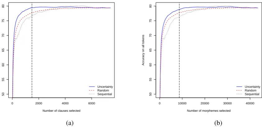
0 2000 4000 6000

50

55

60

65

70

75

80

Number of clauses selected

Accuracy on all tokens

Uncertainty Random Sequential

0 10000 20000 30000 40000

50

55

60

65

70

75

80

Number of morphemes selected

Accuracy on all tokens

Uncertainty Random Sequential

(a) (b)

Figure 1: Learning curves for simulations; (a) clause cost and (b) morphemes cost. The dashed vertical lines indicate (a) #clauses=1485 and (b) #morphemes=8695 (to compare OPER values).

rand

seq uncseq randunc Uspanteko-Clauses 5.86 13.27 7.86 Uspanteko-Morphs 7.47 11.68 4.55

Table 2: OPER values for Uspanteko simulations, comparing clause andmorpheme cost. A

B

indi-cates we compute OPER(A,B).

of the cost metric, but the relative differences in cost-savings are not, which we see when we look at OPER values.

The dashed vertical lines in the two graphs cor-respond to the 20% mark used to calculate OPER values, which are given in Table 2. Most impor-tantly, note the much larger OPER for unc over rand with clause cost (7.86 vs 4.55). Also note that OPER(rand,seq) islowerwith clause cost— this indicates that the beginning portions of the corpus contain longer sentences with more mor-phemes, an accident which overstates how well seqwould likely work in general.

Since rand is unbiased with respect to pick-ing longer sentences, the large increase of OPER(unc,rand) from 4.55 to 7.86 is a clear in-dication of the well-known—but not always at-tended to—tendency of uncertainty sampling to select longer sentences. Consequently, one should at least use sub-sentence cost in order not to over-state the gains from active learning. The annota-tion experiments in the next secannota-tion take this word

rand

seq uncseq randunc Danish 4.58 6.95 2.48 Dutch 21.95 23.68 2.20 English 6.55 8.00 1.56 Swedish 9.56 9.29 -0.30 Uspanteko 7.47 11.68 4.55

Table 3: OPER values formorphemecost for sim-ulations. A

B indicates we compute OPER(A,B).

of caution one step further: even sub-sentence cost (morpheme cost, in our setting) can overestimate gains since the morphemes selected are actually harder to annotate and thus take more time.

Table 3 gives overall percentage error reduc-tions (OPER) between different selection methods based on word/morpheme cost, for each language. For all languages, rand and unc are better than seq. Only in the case of Swedish is there no ben-efit from unc over rand. For Dutch, the large gains over seqfor bothrandandunc accurately reflect the heterogeneity of the underlying Alpino corpus.3 _{Most importantly, for Uspanteko, there} are large reductions fromunctorandtoseq, mir-roring the clear trends in Figure 1b.

These simulations have an unrealistic “perfect” annotator, the corpus. Next, we discuss results with real annotators—who may be fallible or may (reasonably) beg to differ with the corpus analysis.

0 1000 2000 3000 4000

20

30

40

50

60

70

Morphemes annotated

Accuracy on all tokens

Non−Expert, No Suggest, Sequential Non−Expert, Suggest, Random Expert, No Suggest, Sequential Expert, No Suggest, Uncertainty

0 5000 10000 15000 20000 25000

20

30

40

50

60

70

Cumulative annotation time

Accuracy on all tokens

Non−Expert, No Suggest, Sequential Non−Expert, Suggest, Random Expert, No Suggest, Sequential Expert, No Suggest, Uncertainty

(a) (b)

Figure 2: A sample of the learning curves with (a) morpheme cost and (b) time cost. Morpheme cost ranks strategies for a given annotator similarly to time cost, but it gives dramatically different results from time cost when used to compare different annotators.

5 Annotation experiments

With two annotators (expert, non-expert), three selection methods (seq,rand,unc), and two ma-chine labeling settings (ns,ds), we obtain 12 dif-ferent experiments. Each experiment measures ac-curacy in terms of all words and unknown words and cost in terms of clauses, morphemes and time; this produces six views on every experiment. In this paper we focus on one view: accuracy over all words with time-based evaluation of cost.

As with the simulations, clause cost in the an-notation experiments overestimates the cost reduc-tions. For morpheme cost, the annotation experi-ments show that (a) it also overstates cost reduc-tions compared to time, and (b) it can mis-state relative effectiveness when comparing annotators. The big picture. Figure 2 shows curves for four experiments: seq-nsfor both annotators4 _{and the} most effective overall condition for each annota-tor. Figure 2a uses morpheme cost evaluation; on that metric, both annotators appear to be about equally effective with seq-ns and much more ef-fective with machine involvement (uncords) than without. Additionally, the non-expert’s rand-ds appears to beat the expert’sunc-ns. However, the time cost evaluation in Figure 2b tells a dramat-ically different story. Each annotator’s

machine-4_{Recall that sequential annotation is the default mode for} producing IGT, so this strategy is of particular interest.

involved experiment is much better than theirseq -ns, but now the expert’s best is clearly better than the non-expert’s. We see this as clear evidence for the need for cost-sensitive learning over vanilla ac-tive learning (as we do here).5

The non-expert withrand-dscaught up to and surpassed the unaided expert in about six hours total annotation time, and he caught up to her unc-ns curve after 35 hours. This is encourag-ing since often language documentation projects have participants with a wide range of expertise levels, and these results suggest that assistance from machine learning, if done properly, may in-crease the effectiveness of participants with less language-specific expertise. We are also encour-aged, with respect to the effectiveness of active learning, that the expert’s best performance is ob-tained with uncertainty-based selection.

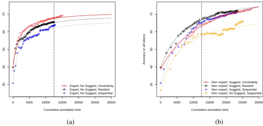
Within annotator comparisons. Figure 3 shows both actual measurements and the fitted nonlinear regression curves used to compute OPER. Figure 3a, the expert without suggestions, exhibits typical active learning behavior similar to that seen in the simulation experiments. Figure 3b,

● ●

● ●

● ●

●●● ●●

●●●●●●● ●●●●

●●●●●●●●●●● ●●●●●●●●●●●●●●●●●●●●●●●●

0 5000 10000 15000 20000 25000 30000

30

40

50

60

70

Cumulative annotation time

Accuracy on all tokens

● _{Expert, No Suggest, Uncertainty}

Expert, No Suggest, Random Expert, No Suggest, Sequential

● ●

● ●

●●●● ●●

●● ●●● ●●●●●●●

●●●● ●●● ●●●●●●

●●●●●●●●●●●●●● ●●●●●●●●

0 5000 10000 15000 20000 25000 30000

30

40

50

60

70

Cumulative annotation time

Accuracy on all tokens

● _{Non−expert, Suggest, Uncertainty}

Non−expert, Suggest, Random Non−expert, Suggest, Sequential Non−expert, No Suggest, Sequential

(a) (b)

Figure 3: Sample measurements and fitted nonlinear regression curves for (a) the expert and (b) the non-expert. Note that the scale is consistent for comparability. The dashed vertical lines indicate 12,500 seconds (about 35 hours), which is the upper limit used in computing OPER values for Table 4.

the non-expertwithsuggestions, shows that in the ds conditions the non-expert was less effective with unc. This is not unexpected: uncertainty selects harder examples that will either take longer to annotate or are easier to get wrong, especially if the annotator trusts the classifier and

especially on examples the classifier is uncertain about. Nonetheless, in alldscases, the non-expert performs better than withseq-ns.

OPER. Table 4 provides OPER values from time 0 to 12,500 seconds (about 35 hours), the minimum amount of annotation time logged in any one of the twelve experiments.6 _{The table mixes} three types of comparison: (1) the boxed values on the diagonal give OPER for the expert versus the non-expert given the same selection and sug-gestion conditions; (2) the upper (right) triangle gives OPER for the expert versus herself for dif-ferent conditions; and (3) the lower (left) trian-gle is the non-expert versus himself. For exam-ple: (1) the expert obtained an 11.52 OPER versus the non-expert when both used rand-ns; (2) the expert obtained a 10.52 OPER by using rand-ds rather thanseq-ns; and (3) the non-expert obtained a 5.93 OPER overrand-nsby usingrand-ds.

A number of patterns emerge. Quite

unsurpris-6_{Stopping at 12,500 seconds ensures a fair comparison,} for example, between the expert and the non-expert because it requires no extrapolation of the expert’s performance.

XXXXXXnon-exp exp seq-ns rand-ns unc-ns seq-ds rand-ds unc-ds seq-ns 15.99 8.85 14.17 6.34 10.52 14.50 rand-ns 13.46 11.52 5.83 -2.76 1.83 6.20 unc-ns 19.20 6.63 10.76 -9.12 -4.25 0.39 seq-ds 10.24 -3.72 -11.09 12.34 4.46 8.72 rand-ds 18.59 5.93 -0.76 9.30 7.67 4.45 unc-ds 11.19 -2.62 -9.91 1.06 -9.09 19.13

Table 4: Overall percentage error reduction (OPER) comparisons, with timing cost. See ex-planation of table in theOPERsubsection.

ingly, the values on the diagonal show that the ex-pert is more effective than the non-exex-pert in all conditions. Also, every other condition is more ef-fective thanseq-ns for both annotators (first row for the expert, first column for the non-expert). unc-ns andrand-ds are particularly effective for the non-expert, giving OPERs of 19.20 and 18.59 overseq-ns, respectively. These reductions, big-ger than the expert’s reductions of 14.17 and 10.52 for the same conditions, considerably reduce the large gap inseq-nseffectiveness between the two annotators (see Figure 2b).

but performs worse when used with unc (-9.91 OPER). Even more striking: the non-expert’s unc-ds is worse than rand-ns (-2.62 OPER), a completely model-free setting. These variations demonstrate the importance of modeling annotator fallibility and sensitivity to cost, as well as char-acteristics of the annotation task itself, if learner-guided selection and suggestion are to be used (Donmez and Carbonell, 2008; Arora et al., 2009).

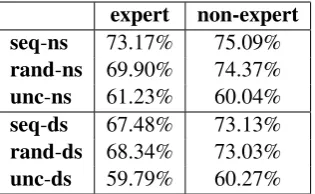
Annotator accuracy. Another factor which must be considered when annotation is done by human annotators (rather than being simulated) is the accuracy of the humans’ labels. Table 5 shows the overall accuracy of the annotators’ la-bels for each condition (after 56 rounds) as mea-sured against the original OKMA annotations. Unsurprisingly,uncselection picks examples that are more difficult to annotate: accuracy for both annotators suffers in bothunc-nsandunc-ds.

It may seem surprising that the non-expert’s ac-curacies are generally higher than the expert’s. The main reason for this is that the non-expert took nearly twice as long to annotate his examples, so each one was done with more care. However, this difference also highlights challenges that arise when we bring active learning into non-simulated annotation contexts. The typical assumption is that gold standard labeled data represents a true, fixed target, against which annotator or machine-predicted labels should be measured. In language documentation, though, the analysis of the lan-guage is continually evolving, and analysis and annotation each inform the other. In fact, the ex-pert recognized (in the morphological segmenta-tion) several linguistic phenomena for which the analysis has changed since the original OKMA an-notations were done. As she changed her analy-ses, her labels diverged from those of the original corpus—another reason for her “lower” accuracy. This is to say that the ground truth of the current OKMA annotations we had to work with can be viewed as one (valid) stage in the iterative reanal-ysis process that language documentation is.

Error analysis. Preliminary analysis of ‘errors’ made by the annotators supports the idea that the results seen in Table 5 are heavily influenced by changes in the expert’s analysis of the lan-guage. Some duplicate clause annotation oc-curred for each annotator, because each of the twelve annotator-selection-suggestion conditions

expert non-expert seq-ns 73.17% 75.09% rand-ns 69.90% 74.37% unc-ns 61.23% 60.04% seq-ds 67.48% 73.13% rand-ds 68.34% 73.03% unc-ds 59.79% 60.27%

Table 5: Overall accuracy of annotators’ labels, measured against OKMA annotations.

drew from the same global set of unlabeled ex-amples. This duplication allows us to measure the consistency of each annotator on labeling such duplicate clauses. Table 6 shows the percentage of morphemes labeled consistently by each anno-tator. Numbers for the expert appear in the top (right) triangle, and for the non-expert in the bot-tom (left) triangle. Overall intra-annotator consis-tency is much higher for the expert (88.38%) than for the non-expert (81.64%), suggesting that the expert maintained a more consistent mental model of the language, but one which disagrees in some areas with the original annotations.

PPP_{non PPP}exp _{seq-ns rand-ns unc-ns seq-ds rand-ds unc-ds} seq-ns — 95.00% (41) 87.10% (56) 92.39% (60) 91.02% (28) 88.83% (51) rand-ns 90.11% (49) — 90.91% (57) 87.57% (35) 90.94% (50) 89.53% (57) unc-ns 80.80% (44) 81.68% (54) — 81.35% (41) 89.10% (40) 87.82% (332) seq-ds 90.00% (54) 87.94% (44) 77.97% (48) — 86.13% (42) 82.14% (42) rand-ds 90.15% (52) 86.64% (45) 79.46% (62) 81.43% (44) — 87.06% (49) unc-ds 84.15% (47) 78.55% (52) 77.68% (328) 78.81% (35) 77.95% (60) —

Table 6: Annotation consistency, expert and non-expert, (number of duplicate clauses, of 560 possible)

PPP_PPP

non exp seq-ns rand-ns unc-ns seq-ds rand-ds unc-ds

seq-ns 69.91% (523) 70.82% (42) 62.42% (48) 72.35% (54) 74.25% (28) 67.82% (47) rand-ns 71.32% (48) 83.94% (39) 66.56% (47) 66.15% (43) 73.75% (42) 67.55% (52) unc-ns 66.31% (48) 67.87% (53) 62.31% (301) 58.87% (51) 73.31% (40) 61.10% (298) seq-ds 73.35% (60) 75.56% (34) 56.39% (37) 60.02% (540) 66.00% (44) 61.01% (36) rand-ds 68.67% (50) 76.40% (63) 66.67% (58) 65.88% (47) 76.33% (42) 66.99% (64) unc-ds 65.41% (50) 67.98% (55) 60.43% (263) 58.13% (38) 70.74% (57) 60.40% (275)

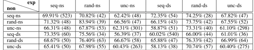
Table 7: IAA: expert v. non-expert, percentage of morphemes in agreement, (number of duplicate clauses, of 560 possible)

6 Conclusion

Through actual annotation experiments that con-trol for several factors, we have evaluated the po-tential of incorporating active learning and label suggestions to speed up morpheme glossing in a realistic language documentation context. Some configurations of learner-guided example selec-tion and machine label suggesselec-tions perform far better than the standard strategy of sequential se-lection without suggestions. However, the effec-tiveness of any given strategy depends on annota-tor expertise. The impact of differences between annotators directly bears on the point made by Donmez and Carbonell (2008) that if cost reduc-tions are to be reliably obtained with active learn-ing techniques, annotators’ fallibility, unreliabil-ity, and sensitivity to cost must be modeled.

Our results suggest some possible prescriptions for tuning techniques according to annotator ex-pertise. However, even if we can estimate a rela-tive level of expertise, following such broad pre-scriptions is unlikely to be more robust than an ap-proach which adapts selection and suggestion to the individual annotator, perhaps working within an annotation group. Indeed, it seems that dealing with variation in annotators/oracles may be more important than devising better selection strategies. The difference in performance due to expertise suggests that using multiple annotators to check relative annotation rate and accuracy of different annotators could be a key ingredient in any

actu-ally deployed active learning system. This could provide for better modeling of individual anno-tators as part of an annotation group they can be compared against, allowing the system, for exam-ple, to throttle active selection if an annotator ap-pears to be too slow or inaccurate.

Another major issue we highlight is the uncer-tainty around the question of whether active learn-ing works in practical applications. Respondents to the survey of Tomanek and Olsson (2009) in-dicated that this uncertainty—will active learn-ing work? what methods or techniques will work best?—is one of the reasons active learning is not widely used in actual annotation. In addition, cre-ating the necessary software infrastructure to build an active learning enabled annotation system— a system which must interface robustly between data, annotator, and machine classifier, yet still be easy to use—is a substantial hurdle. It seems unlikely that there will be much uptake until a) consistent, large cost reductions can be shown in actual annotation studies, and b) appropriate, tun-able, widely-available software exists.

Acknowledgments

References

Shilpa Arora, Eric Nyberg, and Carolyn P. Ros´e. 2009. Estimating annotation cost for active learning in a multi-annotator environment. InProceedings of the NAACL HLT Workshop on Active Learning for Nat-ural Language Processing, pages 18–26, Boulder, CO.

Jason Baldridge and Miles Osborne. 2008. Active learning and logarithmic opinion pools for HPSG parse selection. Natural Language Engineering, 14(2):199–222.

Sabine Buchholz and Erwin Marsi. 2006. CoNLL-X Shared Task on Multilingual Dependency Parsing. In Proceedings of the Tenth Conference on Com-putational Natural Language Learning (CoNLL-X), pages 149–164, New York City, June. Association for Computational Linguistics.

David A. Cohn, Zoubin Ghahramani, and Michael I. Jordan. 1995. Active learning with statistical mod-els. In G. Tesauro, D. Touretzky, and T. Leen, ed-itors, Advances in Neural Information Processing Systems, volume 7, pages 705–712. The MIT Press. David Crystal. 2000. Language Death. Cambridge

University Press, Cambridge.

James R. Curran and Stephen Clark. 2003. Investigat-ing GIS and smoothInvestigat-ing for maximum entropy tag-gers. InProceedings of the 10th Conference of the European Association for Computational Linguis-tics, pages 91–98.

Pinar Donmez and Jaime G. Carbonell. 2008. Proac-tive learning: Cost-sensiProac-tive acProac-tive learning with multiple imperfect oracles. In Proceedings of CIKM08, Napa Valley, CA.

Ben Hachey, Beatrice Alex, and Markus Becker. 2005. Investigating the effects of selective sampling on the annotation task. In Proceedings of the 9th Confer-ence on Computational Natural Language Learning, Ann Arbor, MI.

Robbie A. Haertel, Kevin D. Seppi, Eric K. Ringger, and James L. Carroll. 2008. Return on invest-ment for active learning. InProceedings of the NIPS Workshop on Cost-Sensitive Learning.

Mitchell P. Marcus, Beatrice Santorini, and Mary Ann Marcinkiewicz. 1993. Building a large annotated corpus of English: the Penn Treebank. Computa-tional linguistics, 19:313–330.

Prem Melville and Raymond J. Mooney. 2004. Di-verse ensembles for active learning. In Proceed-ings of the 21st International Conference on Ma-chine Learning, pages 584–591, Banff, Canada. Grace Ngai and David Yarowsky. 2000. Rule

writ-ing or annotation: cost-efficient resource usage for base noun phrase chunking. InProceedings of the 38th Annual Meeting of the Association for Compu-tational Linguistics, pages 117–125, Hong Kong.

Alexis Palmer, Taesun Moon, and Jason Baldridge. 2009. Evaluating automation strategies in language documentation. InProceedings of the NAACL HLT 2009 Workshop on Active Learning for Natural Lan-guage Processing, pages 36–44, Boulder, CO. Telma Can Pixabaj, Miguel Angel Vicente M´endez,

Mar´ıa Vicente M´endez, and Oswaldo Ajcot Dami´an. 2007. Text Collections in Four Mayan Languages. Archived in The Archive of the Indigenous Lan-guages of Latin America.

Adwait Ratnaparkhi. 1998. Maximum Entropy Models for Natural Language Ambiguity Resolution. Ph.D. thesis, University of Pennsylvania, Philadelphia, PA. Christian Ritz and Jens Carl Streibig. 2008. Nonlinear

Regression with R. Springer.

Burr Settles, Mark Craven, and Lewis Friedland. 2008. Active learning with real annotation costs. In Pro-ceedings of the NIPS Workshop on Cost-Sensitive Learning.

Burr Settles. 2009. Active learning literature survey. Technical Report Computer Sciences Technical Re-port 1648, University of Wisconsin-Madison. Rion Snow, Brendan O’Connor, Daniel Jurafsky, and

Andrew Y. Ng. 2008. Cheap and fast - but is it good? Evaluating non-expert annotations for natu-ral language tasks. InProceedings of EMNLP 2008, pages 254–263.

Katrin Tomanek and Fredrik Olsson. 2009. A Web Survey on the Use of Active learning to support an-notation of text data. InProceedings of the NAACL HLT Workshop on Active Learning for Natural Lan-guage Processing, pages 45–48, Boulder, CO. Sudheendra Vijayanarasimhan and Kristen Grauman.