Structure Learning for Neural Module Networks

1

Structure Learning for Neural Module Networks

Vardaan Pahuja∗ Jie Fu†‡ Sarath Chandar†§ Christopher J. Pal†‡

†_Mila §_{Université de Montréal}

‡_{Polytechnique Montréal The Ohio State University}

Abstract

Neural Module Networks, originally proposed for the task of visual question answering, are a class of neural network architectures that in-volve human-specified neural modules, each designed for a specific form of reasoning. In current formulations of such networks only the parameters of the neural modules and/or the or-der of their execution is learned. In this work, we further expand this approach and also learn the underlying internal structure of modules in terms of the ordering and combination of sim-ple and elementary arithmetic operators. We utilize a minimum amount of prior knowledge from the human-specified neural modules in the form of different input types and arithmetic operators used in these modules. Our results show that one is indeed able to simultaneously learn both internal module structure and mod-ule sequencing without extra supervisory sig-nals for module execution sequencing. With this approach, we report performance compa-rable to models using hand-designed modules. In addition, we do a analysis of sensitivity of the learned modules w.r.t. the arithmetic oper-ations and infer the analytical expressions of the learned modules.

1 Introduction

Designing general purpose reasoning modules is one of the central challenges in artificial intelli-gence. Neural Module Networks (Andreas et al., 2016b) were introduced as a general purpose vi-sual reasoning architecture and have been shown to work well for the task of visual question answering (Antol et al., 2015;Malinowski and Fritz, 2014; Ren et al.,2015b,a). They use dynamically com-posable modules which are then assembled into a layout based on syntactic parse of the question.

∗

Corresponding author: Vardaan Pahuja <[email protected]> Work done when the author was a stu-dent at Mila, Université de Montréal.

The modules take as input the images or the at-tention maps1_{and return attention maps or labels}

as output. In (Hu et al.,2017), the layout predic-tion is relaxed by learning a layout policy with a sequence-to-sequence RNN. This layout policy is jointly trained along with the parameters of the modules. The model proposed in (Hu et al.,2018) avoids the use of reinforcement learning to train the layout predictor, and uses soft program execution to learn both layout and module parameters jointly.

A fundamental limitation of these previous ular approaches to visual reasoning is that the mod-ules need to be hand-specified. This might not be feasible when one has limited knowledge of the kinds of questions or associated visual reason-ing required to solve the task. In this work, we present an approach to learn the module structure, along with the parameters of the modules in an end-to-end differentiable training setting. Our pro-posed model, Learnable Neural Module Network (LNMN), learns the structure of the module, the parameters of the module, and the way to compose the modules based on just the regular task loss. Our results show that we can learn the structure of the modules automatically and still perform com-parably to hand-specified modules. We want to highlight the fact that our goal in this paper is not to beat the performance of the hand-specified mod-ules since they are specifically engineered for the task. Instead, our goal is to explore the possibility of designing general-purpose reasoning modules in an entirely data-driven fashion.

2 Background

In this section, we describe the working of the Stack-NMNmodel (Hu et al.,2018) as our proposed LNMN model uses this as the base model. The

Stack-NMNmodel is an end-to-end differentiable model for the task of Visual Question Answering and Referential Expression Grounding (Rohrbach et al., 2016). It addresses a major drawback of prior visual reasoning models in the literature that compositional reasoning is implemented without the need of supervisory signals for composing the layout at training time. It consists of several hand-specified modules (namely Find, Transform, And, Or, Filter, Scene, Answer, Compare and NoOp) which are parameterized, differentiable, and imple-ment common routines needed in visual reasoning and learns to compose them without strong supervi-sion. The implementation details of these modules are given in AppendixA.2(see Table8). The dif-ferent sub-components of the Stack-NMN model are described below.

2.1 Module Layout Controller

The structure of the controller is similar to the one proposed in (Hudson and Manning, 2018). The controller first encodes the question using a bi-directional LSTM (Hochreiter and Schmidhuber, 1997). Let [h1,h2, ...,hS]denote the output of

Bi-LSTM at each time-step of the input sequence of question words. Letqdenote the concatenation of final hidden state of Bi-LSTM during the for-ward and backfor-ward passes.qcan be considered as the encoding of the entire question. The controller executes the modules iteratively forT times. At each time-step, the updated query representationu

is obtained as:

u=W2[W1(t)q+b1;ct−1] +b2

where W₁(t) ∈ Rd×d, W2 ∈ Rd×2d, b1 ∈ Rd,

b2 ∈ Rd are controller parameters. ct−1 is the textual parameter from the previous time step. The controller has two outputs viz. the textual param-eter at stept(denoted byct) and the attention on

each module (denoted by vectorw(t)). The con-troller first predicts an attentioncvt,son each of the

words of the question and then uses this attention to do a weighted average over the outputs of the Bi-LSTM.

cvt,s=sof tmax(W3(uhs))

ct= S

X

s=1

cvt,s·hs

where,W3 ∈R1×dis another controller parameter.

The attention on each modulew(t)is obtained by

feeding the query representation at each time-step to a Multi-layer Perceptron (MLP).

w(t)=sof tmax(M LP(u;θM LP))

2.2 Operation of Memory Stack for storing attention maps

In order to answer a visual reasoning question, the model needs to execute modules in a tree-structured layout. In order to facilitate this sort of composi-tional behavior, a differentiable memory pool to store and retrieve intermediate attention maps is used. A memory stack (with length denoted byL) storesH×W dimensional attention maps, where

H andW are the height and width of image fea-ture maps respectively. Depending on the number of attention maps required as input by the mod-ule, it pops them from the stack and later pushes the result back to the stack. The model performs soft module execution by executing all modules at each time step. The updated stack and stack

Data:Question (string), Image features (I) Encode the input question into

d-dimensional sequence[h1,h2, ...,hS]

using Bidirectional LSTM.

A(0)_{←Initialize the memory stack(A;p)}

with uniform image attention and set the stack pointerpto point at the bottom of the stack (one-hot vector with1in the1st

dim.).

foreach time-step t = 0, 1, ...., (T-1)do

u=W2[W1(t)q+b1;ct−1] +b2;

w(t)=sof tmax(M LP(u;θM LP));

cvt,s =sof tmax(W3(uhs)); ct=PS_s=1cvt,s·hs

forevery modulem∈M do Produce updated stack and stack

pointer:(A(mt), p(mt)) =

run-module(m, A(t), p(t),ct,I);

end

A(t+1) =P

m∈MA (t) m ·w(mt);

p(t+1) =sof tmax(P

m∈Mp (t) m ·w(mt))

end

Algorithm 1: Operation of Module Layout Controller and Memory Stack.

equations below:

(A(_mt), p(_mt)) =run-module(m, A(t), p(t))

A(t+1)= X m∈M

A(_mt)·w(_mt)

p(t+1)=sof tmax(X m∈M

p(_mt)·w(_mt))

Here, A(mt) and p(mt) denote the stack and stack

pointer respectively, after executing modulemat time-stept.A(t)andp(t)denote the stack and stack pointer obtained after the weighted average of those corresponding to all modules at previous time-step

(t−1). The working of module layout controller and its interfacing with memory stack is illustrated in Algorithm1. The implementation details of op-eration of the stack are shown in Appendix (see Algorithm3).

2.3 Final Classifier

At each time-step of module execution, the weighted average of output of theAnswermodules is called memory features (denoted by fmem(t) =

P

m∈ans. moduleo (t)

mw(mt)). Here,o(mt)denotes the

out-put of modulemat timet. The memory features are given as one of the inputs to theAnswer mod-ules at the next time-step. The memory features at the final time-step are concatenated with the question representation, and then fed to an MLP to obtain the logits.

3 Learnable Neural Module Networks

In this section, we introduce Learnable Neural Module Networks (LNMNs) for visual reasoning, which extends Stack-NMN. However, the modules in LNMN are not hand-specified. Rather, they are generic modules as specified below.

3.1 Structure of the Generic Module

The cell(see Figures1 and2) denotes a generic module, which we suppose can span all the re-quired modules for a visual reasoning task. Each cell contains a certain number of nodes. The func-tion of a node (denoted by O) is to perform a weighted sum of outputs of different arithmetic op-erations applied on the input feature mapsx1 and

x2. Letα

0

=σ(α)denote the output of softmax

function applied to the vectorαsuch that

O(x1,x2) =α

0

1∗min(x1,x2)

+α0₂∗max(x1,x2) +α

0

3∗(x1+x2)+

α0₄∗(x1x2) +α

0

5∗choose1(x1,x2)

+α0₆∗choose2(x1,x2)

All of the above operations (min, max, +, ) are element-wise operations. The last two non-standard functions are defined as:

choose1(x1,x2) = x1 andchoose2(x1,x2) =

x2.

We consider two broad kinds of modules: (i) Attention moduleswhich output an attention map (ii)Answer moduleswhich output memory features to be stored in the memory. Among each of these two categories, there is a finer categorization:

3.1.1 Generic Module with 3 inputs

This module type receives 3 inputs (i.e. image features, textual parameter, and a single attention map) and produces a single output. The first node receives input from the image feature (I) and the attention map (popped from the memory stack). The second node receives input from the textual parameter followed by a linear layer (W1ctxt), and

the output of the first node.

3.1.2 Generic Module with 4 inputs

This module type receives 4 inputs (i.e. image fea-tures, textual parameter and two attention maps) and produces a single output. The first node re-ceives the two attention maps, each of which are popped from the memory stack, as input. The sec-ond node receives input from the image features along with the output of the first node. The third node receives input from the textual parameter fol-lowed by a linear layer, and the output of the second node.

Figure 1: Attention Module schematic diagram (3 inputs).

Figure 2: Attention Module schematic diagram (4 inputs).

3.2 Overall structure

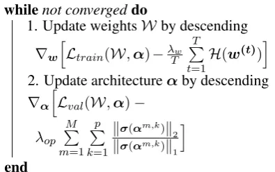
The structure of our end-to-end model extends Stack-NMNin that we specify each module in terms of the generic module (defined in Section3.1). We experiment with three model ablations in terms of number of modules for each type being used. See Table3for details2. We train the module structure parameters (denoted byα =nαm,k_i o6

i=1 for k th

node of modulem) and the weight parameters (W) by adopting alternating gradient descent steps in ar-chitecture and weight spaces respectively. For a par-ticular epoch, the gradient step in weight space is performed on each training batch, and the gradient step in architecture space is performed on a batch randomly sampled from the validation set. This is done to ensure that we find an architecture corre-sponding to the modules which has a low validation loss on the updated weight parameters. This is in-spired by the technique used in (Liu et al.,2018) to learn monolithic architectures like CNNs and RNNs in terms of basic building blocks (orcells). Algorithm2illustrates the training algorithm. Here, Ltrain(W,α)andLval(W,α)denote the training

2_{1 NoOp module is included by default in all ablations.}

whilenot convergeddo

1. Update weightsWby descending

∇_whL_train(W,α)−λw T

T

P

t=1

H(w(t))i

2. Update architectureαby descending ∇α

h

Lval(W,α)−

λop M

P

m=1 p

P

k=1

kσ(αm,k_)k

2

kσ(αm,k_)k

1

i

end

Algorithm 2:Training Algorithm for LNMN Modules. Here, α denotes the collection of

module network parameters i.e. n

αm,k_i o6

i=1

loss and validation loss on the combination of pa-rameters(W,α)respectively. For the gradient step on the training batch, we add an additional loss term to initially maximize the entropy ofw(t)and gradually anneal the regularization coefficient (λw)

to the opposite sign (which minimizes the entropy ofw(t)towards the end of training). The value of

λw varies linearly from1.0to 0.0in the first 20

epochs and then steeply decreases to−1.0in next 10 epochs. The trend of variation ofλw is shown

in Appendix (see Figure5). For the gradient steps in the architecture space, we add an additional loss term (l_l21 =

kσ(α)k₂

kσ(α)k₁) (Hurley and Rickard,2009) to encourage the sparsity of module structure parame-ters (α) after the softmax activation.

4 Experiments

We train our model on the CLEVR visual rea-soning task. CLEVR (Johnson et al., 2017a) is a synthetic dataset for visual reasoning contain-ing around 700K examples, and has become the standard benchmark to test visual reasoning mod-els. It contains questions that test visual reasoning abilities such as counting, comparing, logical rea-soning based on 3D shapes like cubes, spheres, and cylinders of varied shades. A typical example ques-tion and image pair from this dataset is given in Appendix (see Figure4). The results on CLEVR test set are reported in Table1. Some ablations of the model are shown in Table 2. We use the pre-trained CLEVR model to fine-tune the model on CLEVR-Humans dataset. The latter is a dataset of challenging human-posed questions based on a much larger vocabulary on the same CLEVR images. The corresponding results are shown in Table1(see last column). In addition, we exper-iment on VQA v1 (Antol et al.,2015) and VQA v2 (Goyal et al., 2017) which are VQA datasets containing natural images. The results for VQA v1 and VQA v2 are shown in Table4.

The detailed accuracy for each question sub-type for the VQA datasets is given in Appendix A.4 (see Tables 9 and 10). We use Adam (Kingma and Ba,2014) as the optimizer for the weight pa-rameters with a learning rate of1e−4,(β1, β2) = (0.9,0.999)and no weight decay. For the module network parameters, we use the same optimizer with a different learning rate 3e−4, (β1, β2) = (0.5,0.999)and a weight decay of1e−3. The value ofλopis set to1.0. The code for implementation

of our model is available online3.

4.1 Results

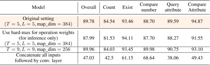
The comparison of CLEVR overall accuracy shows that our model (LNMN (9 modules)) receives only a slight dip (1.53%) compared to the Stack-NMN model. We also experiment with other variants of our model in which we increase the number ofAnswermodules (LNMN (11 modules)) and/or Attention modules (LNMN (14 modules)). The LNMN (11 modules) model performs better than the other two ablations (0.89%accuracy drop w.r.t. the Stack-NMN model). For the ‘Count’ and ‘Com-pare Numbers’ sub-category of questions, all of the 3 variants perform consistently better than the Stack-NMN model. In case of CLEVR-Humans dataset, the accuracy drop is a modest1.71%. Even for the natural image VQA datasets, our approach has comparable results with the Stack-NMN model. The results clearly show that the modules learned by our model (in terms of elementary arithmetic op-erations) perform approximately as well as the ones specified in the Stack-NMN model (that contains hand-designed modules which were tailor-made for the CLEVR dataset). The results from the ab-lations in Table2show that a naive concatenation of all inputs to a module (orcell) results in a poor performance (around 47%). Thus, the structure we propose to fuse the inputs plays a key role in model performance. When we replace theαvector for each node by a one-hot vector during inference, the drop in accuracy is only1.79%which shows that the learned distribution over operation weights peaks over a specific operation which is desirable.

4.2 Measuring the sensitivity of modules

We use an attribution technique called Integrated Gradients (Sundararajan et al.,2017) to study the impact of module structure parameters (denoted

by nαm,k_i o6

i=1 for k

th _{node of module m) on}

the probability distribution in the last layer of LNMN model. Let I_j and qj denote the

(im-age, question) pairs for the jth example. Let

F(I_j,qj,α)denote the function that assigns the

probability corresponding to the correct answer in-dex in the softmax distribution. Here,αm,k_i denotes the module network parameter for theithoperator in kth node of modulem. Then, the attribution of[αm₁ , αm₂ , αm₃ , αm₄ , αm₅ , α₆m](summed across all nodesk = 1, ..., pfor a particular modulemand

Model CLEVR Count Exist Compare Query Compare CLEVR Overall Numbers Attribute Attribute Humans

Human (Johnson et al.,2017b) 92.6 86.7 96.6 86.5 95.0 96.0 -Q-type baseline (Johnson et al.,2017b) 41.8 34.6 50.2 51.0 36.0 51.3 -LSTM (Johnson et al.,2017b) 46.8 41.7 61.1 69.8 36.8 51.8 36.5 CNN+LSTM (Johnson et al.,2017b) 52.3 43.7 65.2 67.1 49.3 53.0 43.2 CNN+LSTM+SA+MLP (Johnson et al.,2017a) 73.2 59.7 77.9 75.1 80.9 70.8 57.6 N2NMN* (Hu et al.,2017) 83.7 68.5 85.7 84.9 90.0 88.7 -PG+EE (700K prog.)* (Johnson et al.,2017b) 96.9 92.7 97.1 98.7 98.1 98.9 -CNN+LSTM+RN‡(Santoro et al.,2017) 95.5 90.1 97.8 93.6 97.9 97.1 -CNN+GRU+FiLM (Perez et al.,2017) 97.7 94.3 99.1 96.8 99.1 99.1 75.9 MAC (Hudson and Manning,2018) 98.9 97.1 99.5 99.1 99.5 99.5 81.5 TbD (Mascharka et al.,2018) 99.1 97.6 99.2 99.4 99.5 99.6

-Stack-NMN (9 mod.)†(Hu et al.,2018) 91.41 81.78 95.78 85.23 95.45 95.68 68.06

LNMN (9 modules) 89.88 84.28 93.74 89.63 89.64 94.84 66.35 LNMN (11 modules) 90.52 84.91 95.21 91.06 90.03 94.97 65.68 LNMN (14 modules) 90.42 84.79 95.52 90.52 89.73 95.26 65.86

Table 1: CLEVR and CLEVR-Humans Accuracy by baseline methods and our models. (*) denotes use of extra su-pervision through program labels. (‡) denotes training from raw pixels.†Accuracy figures for our implementation of Stack-NMN.

Model Overall Count Exist Compare number

Query attribute

Compare Attribute

Original setting

(T = 5, L= 5,map_dim= 384) 89.78 84.54 93.46 88.70 89.59 94.87

Use hard-max for operation weights (for inference only)

(T = 5, L= 5,map_dim= 384)

87.99 81.53 94.11 87.70 88.27 91.55

T = 9, L= 9,map_dim= 256 89.96 84.03 93.45 89.98 90.75 93.10 Concatenate all inputs

followed by conv. layer 47.03 42.5 61.15 68.64 38.06 49.43

Table 2: Model Ablations for LNMN (CLEVR Validation set performance). The term ‘map_dim’ refers to the dimension of feature representation obtained at the input or output of each node of cell.

Model

Attn. modules (3 input)

Attn. modules (4 input)

Ans. modules (3 input)

Ans. modules (4 input)

LNMN (9) 4 2 1 1 LNMN (11) 4 2 2 2 LNMN (14) 5 4 2 2

Table 3: Number of modules of each type for different model ablations.

Model VQA v2 VQA v1

Stack-NMN 58.23 59.84 LNMN (9 modules) 54.85 57.67

Table 4: Test Accuracy on Natural Image VQA datasets

over all examples) is defined as:

IG(αm_i ) = N

X

j=1 p

X

k=1

(αm,k_i −(αm,k_i )0)×

Z 1

ξ=0

∂F(I_j,qj,(1−ξ)×(αm,ki ) 0

+ξ×αm,k_i )

∂α_im,k

Please note that attributions are defined relative to an uninformative input called the baseline. We use a vector of all zeros as the baseline (denoted by (αm,k_i )0). Table 5 shows the results for this experiment.

Module ID Module type min max sum product choose_1 choose_2

0 Attn. (3 input) 6.3e4 2.7e4 3.6e4 1.1e5 5.1e4 1.6e4 1 Attn. (3 input) 4.4e4 1.8e4 6.2e4 1.4e4 2.8e4 1.7e5 2 Attn. (3 input) 7.0e4 3.3e4 3.8e4 1.1e5 5.2e4 1.5e4 3 Attn. (3 input) 8.6e3 6.2e4 1.7e4 1.8e4 4.7e4 3.0e4 4 Attn. (4 input) 4.5e4 3.2e4 7.6e4 1.7e4 3.6e4 2.1e5 5 Attn. (4 input) 1.1e5 5.6e5 2.3e5 8.5e3 2.8e4 1.8e5 6 Ans. (3 input) 2.1e6 4.3e6 4.4e6 8.3e6 2.3e6 4.9e5 7 Ans. (4 input) 1.2e5 5.8e4 1.7e5 5.2e3 1.0e5 4.5e5

Table 5: Analysis of gradient attributions ofαparameters corresponding to each module (LNMN (9 modules)), summed across all examples of CLEVR validation set.

attention maps to produce new feature maps which are used as input by theAnswermodules.

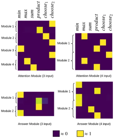
Figure 3: Visualization of module structure parameters (LNMN (11 modules)). For each module, each row de-notes theα0 =σ(α)parameters of the corresponding node.

4.3 Visualization of module network parameters

In order to better interpret the individual contribu-tions from each of the arithmetic operators to the modules, we plot them as color-maps for each type of module. The resulting visualizations are shown in Figure3 for LNMN (11 modules). It is clear from the figure that the operation weights (orα0 pa-rameter) are approximately one-hot for each node. This is necessary in order to learn modules which act as composition of elementary operators on input feature maps rather than a mixture of operations at

each node. The corresponding visualizations for LNMN (9 modules) and LNMN (14 modules) are given in Figure8and Figure9respectively (all of which are given in the AppendixA.3). The analyti-cal expressions of modules learned by LNMN (11 modules) are shown in Table6. The diversity of modules as given in their equations indicates that distinct modules emerge from training.

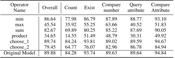
4.4 Measuring the role of individual arithmetic operators

Each module (akacell) contains nodes which in-volves use of six elementary arithmetic opera-tions (i.e. min,max,sum,product,choose_1and choose_2). We zero out the contribution to the node output for one of the arithmetic operations for all nodes in all modules and observe the degra-dation in the CLEVR validegra-dation accuracy4. The results of this study are shown in Table 7. The trend of overall accuracy shows that removingmax andproductoperators results in maximum drop in overall accuracy (∼ 50%). Other operators like min,sumandchoose_1result in minimal drop in overall accuracy.

5 Related Work

Neural Architecture Search: Neural Architecture Search (NAS) is a technique to automatically learn the structure and connectivity of neural networks rather than training human-designed architectures. In (Zoph and Le, 2016), a recurrent neural net-work (RNN) based controller is used to predict the hyper-parameters of a CNN such as number of filters, stride, kernel size etc. They used RE-INFORCE (Williams,1992) to train the controller

4_{The CLEVR test set ground truth answers are not} pub-lic, so we use the validation set instead. However, Table1

Module type Module implementation

Attention (3 inputs)

O(img, a, ctxt) =conv2(choose2(conv1(I), a)W1ctxt) =conv2(aW1ctxt) O(img, a, ctxt) =conv2(choose2(choose1(conv1(I), a), W1ctxt)) =conv2(W1ctxt) O(img, a, ctxt) =conv2(choose2(min(conv1(I), a), W1ctxt)) =conv2(W1ctxt) O(img, a, ctxt) =conv2(max(conv1(I), a) +W1ctxt))

Attention (4 inputs)

O(img, a1, a2, ctxt) =conv2(choose1(max(a1, a2), conv1(I))W1ctxt))

=conv2(max(a1, a2)W1ctxt)

O(img, a1, a2, ctxt) =conv2(max(choose2(a1, a2), conv1(I))W1ctxt))

=conv2(max(a2, conv1(I))W1ctxt))

Answer (3 inputs)

O(img, a, ctxt) =W2[Pmin(conv1(I), a)W1ctxt, W1ctxt, fmem] O(img, a, ctxt) =W2[Pmin((conv1(I)a), W1ctxt), W1ctxt, fmem]

Answer (4 inputs)

O(img, a1, a2, ctxt) =W2[Pmin((min(a1, a2)conv1(I)), W1ctxt), W1ctxt, fmem] O(img, a1, a2, ctxt) =W2[P((min(a1, a2) +conv1(I))W1ctxt), W1ctxt, fmem]

Table 6: Analytical expression of modules learned by LNMN (11 modules). In the above equations,P_denotes sum over spatial dimensions of the feature tensor.

Operator

Name Overall Count Exist

Compare number

Query attribute

Compare Attribute min 86.64 77.98 86.79 87.89 88.77 93.10 max 45.54 35.92 55.25 63.66 40.52 51.83 sum 82.67 69.89 80.25 85.22 87.69 90.05 product 34.65 14.55 51.49 48.79 30.31 49.92 choose_1 89.74 84.24 93.81 89.02 89.59 94.67 choose_2 79.45 64.77 76.07 82.96 86.78 84.94 Original Model 89.88 84.28 93.74 89.63 89.64 94.84

Table 7: Analysis of performance drop with removing operators from a trained model (LNMN 9 modules) on CLEVR validation set.

with validation set accuracy as the reward signal. As an alternative to reinforcement learning, evolu-tionary algorithms (Stanley,2017) have been used to perform architecture search in (Real et al.,2017; Miikkulainen et al.,2019;Liu et al.,2017;Real et al.,2018). Recently, (Liu et al.,2018) proposed DARTS, a differentiable approach to perform archi-tecture search and reported success in discovering high-performance architectures for both image clas-sification and language modeling. Our approach for learning the structure of modules is inspired by DARTS. (Kirsch et al.,2018) proposes an EM style algorithm to learn black-box modules and their lay-out for image recognition and language modeling tasks.

Visual Reasoning Models: Among the end-to-end models for the task of visual reasoning, FiLM (Perez et al.,2017) uses Conditional Batch Normal-ization (CBN) (De Vries et al.,2017;Dumoulin et al.,2017) to modulate the channels of input con-volutional features in a residual block. (Hudson and Manning,2018) obtains the features by iteratively applying a Memory-Attention-Control (MAC) cell that learns to retrieve information from the image and aggregate the results into a recurrent memory.

results in more interpretability of the modules since they perform specific functions.

Visual Question Answering: Visual question answering requires a learning model to answer so-phisticated queries about visual inputs. Significant progress has been made in this direction to design neural networks that can answer queries about im-ages. This can be attributed to the availability of relevant datasets which capture real-life images like DAQUAR (Malinowski and Fritz,2014), COCO-QA (Ren et al.,2015a) and most recently VQA (v1 (Antol et al.,2015) and v2 (Goyal et al., 2017)). The most common approaches (Ren et al.,2015b; Noh et al.,2016) to this problem include construc-tion of a joint embedding of quesconstruc-tion and image and treating it as a classification problem over the most frequent set of answers. Recent works (Jabri et al.,2016;Johnson et al.,2017a) have shown that the neural networks tend to exploit biases in the datasets without learning how to reason.

6 Conclusion

We have presented a differentiable approach to learn the modules needed in a visual reasoning task automatically. With this approach, we obtain results comparable to an analogous model in which modules are hand-specified for a particular visual reasoning task. In addition, we present an exten-sive analysis of the degree to which each module influences the prediction function of the model, the effect of each arithmetic operation on overall accu-racy and the analytical expressions of the learned modules. In the future, we would like to benchmark this generic learnable neural module network with various other visual reasoning and visual question answering tasks.

References

Jacob Andreas, Marcus Rohrbach, Trevor Darrell, and Dan Klein. 2016a. Learning to compose neural networks for question answering. arXiv preprint

arXiv:1601.01705.

Jacob Andreas, Marcus Rohrbach, Trevor Darrell, and Dan Klein. 2016b. Neural module networks. In Pro-ceedings of the IEEE Conference on Computer Vi-sion and Pattern Recognition, pages 39–48.

Stanislaw Antol, Aishwarya Agrawal, Jiasen Lu, Mar-garet Mitchell, Dhruv Batra, C. Lawrence Zitnick, and Devi Parikh. 2015. VQA: Visual Question An-swering. InInternational Conference on Computer Vision (ICCV).

Harm De Vries, Florian Strub, Jérémie Mary, Hugo Larochelle, Olivier Pietquin, and Aaron C Courville. 2017. Modulating early visual processing by lan-guage. InAdvances in Neural Information Process-ing Systems, pages 6594–6604.

Vincent Dumoulin, Jonathon Shlens, and Manjunath Kudlur. 2017. A learned representation for artistic style. Proc. of ICLR.

Yash Goyal, Tejas Khot, Douglas Summers-Stay, Dhruv Batra, and Devi Parikh. 2017. Making the V in VQA matter: Elevating the role of image under-standing in Visual Question Answering. In Confer-ence on Computer Vision and Pattern Recognition

(CVPR).

Sepp Hochreiter and Jürgen Schmidhuber. 1997. Long short-term memory. Neural computation, 9(8):1735–1780.

Ronghang Hu, Jacob Andreas, Trevor Darrell, and Kate Saenko. 2018. Explainable neural computation via stack neural module networks. InProceedings of the

European Conference on Computer Vision (ECCV),

pages 53–69.

Ronghang Hu, Jacob Andreas, Marcus Rohrbach, Trevor Darrell, and Kate Saenko. 2017. Learning to reason: End-to-end module networks for visual question answering.CoRR, abs/1704.05526, 3.

Drew A Hudson and Christopher D Manning. 2018. Compositional attention networks for machine rea-soning.arXiv preprint arXiv:1803.03067.

Niall Hurley and Scott Rickard. 2009. Comparing mea-sures of sparsity. IEEE Transactions on Information

Theory, 55(10):4723–4741.

Allan Jabri, Armand Joulin, and Laurens van der Maaten. 2016. Revisiting visual question answering baselines. InEuropean conference on computer vi-sion, pages 727–739. Springer.

compositional language and elementary visual rea-soning. InComputer Vision and Pattern Recognition

(CVPR), 2017 IEEE Conference on, pages 1988–

1997. IEEE.

Justin Johnson, Bharath Hariharan, Laurens van der Maaten, Judy Hoffman, Li Fei-Fei, C Lawrence Zit-nick, and Ross Girshick. 2017b. Inferring and exe-cuting programs for visual reasoning. InICCV.

Diederik P Kingma and Jimmy Ba. 2014. Adam: A method for stochastic optimization. arXiv preprint arXiv:1412.6980.

Louis Kirsch, Julius Kunze, and David Barber. 2018. Modular networks: Learning to decompose neural computation. In Advances in Neural Information

Processing Systems, pages 2414–2423.

Hanxiao Liu, Karen Simonyan, Oriol Vinyals, Chrisan-tha Fernando, and Koray Kavukcuoglu. 2017. Hi-erarchical representations for efficient architecture search. arXiv preprint arXiv:1711.00436.

Hanxiao Liu, Karen Simonyan, and Yiming Yang. 2018. Darts: Differentiable architecture search.

arXiv preprint arXiv:1806.09055.

Mateusz Malinowski and Mario Fritz. 2014. A multi-world approach to question answering about real-world scenes based on uncertain input. InAdvances

in neural information processing systems, pages

1682–1690.

David Mascharka, Philip Tran, Ryan Soklaski, and Ar-jun Majumdar. 2018. Transparency by design: Clos-ing the gap between performance and interpretabil-ity in visual reasoning.2018 IEEE/CVF Conference

on Computer Vision and Pattern Recognition, pages

4942–4950.

Risto Miikkulainen, Jason Liang, Elliot Meyerson, Aditya Rawal, Daniel Fink, Olivier Francon, Bala Raju, Hormoz Shahrzad, Arshak Navruzyan, Nigel Duffy, et al. 2019. Evolving deep neural networks. In Artificial Intelligence in the Age of Neural

Net-works and Brain Computing, pages 293–312.

Else-vier.

Hyeonwoo Noh, Paul Hongsuck Seo, and Bohyung Han. 2016. Image question answering using con-volutional neural network with dynamic parameter prediction. InProceedings of the IEEE conference

on computer vision and pattern recognition, pages

30–38.

Ethan Perez, Florian Strub, Harm de Vries, Vincent Du-moulin, and Aaron C. Courville. 2017.Film: Visual reasoning with a general conditioning layer. CoRR, abs/1709.07871.

Esteban Real, Alok Aggarwal, Yanping Huang, and Quoc V Le. 2018. Regularized evolution for im-age classifier architecture search. arXiv preprint

arXiv:1802.01548.

Esteban Real, Sherry Moore, Andrew Selle, Saurabh Saxena, Yutaka Leon Suematsu, Jie Tan, Quoc Le, and Alex Kurakin. 2017. Large-scale evolution of image classifiers. arXiv preprint arXiv:1703.01041.

Mengye Ren, Ryan Kiros, and Richard Zemel. 2015a. Exploring models and data for image question an-swering. InAdvances in neural information process-ing systems, pages 2953–2961.

Mengye Ren, Ryan Kiros, and Richard Zemel. 2015b. Image question answering: A visual semantic em-bedding model and a new dataset. Proc. Advances in Neural Inf. Process. Syst, 1(2):5.

Anna Rohrbach, Marcus Rohrbach, Ronghang Hu, Trevor Darrell, and Bernt Schiele. 2016. Ground-ing of textual phrases in images by reconstruction.

InEuropean Conference on Computer Vision, pages

817–834. Springer.

Adam Santoro, David Raposo, David G Barrett, Ma-teusz Malinowski, Razvan Pascanu, Peter Battaglia, and Timothy Lillicrap. 2017. A simple neural net-work module for relational reasoning. InAdvances

in neural information processing systems, pages

4967–4976.

Kenneth O Stanley. 2017. Neuroevolution: A different kind of deep learning.

Mukund Sundararajan, Ankur Taly, and Qiqi Yan. 2017. Axiomatic attribution for deep networks. arXiv preprint arXiv:1703.01365.

Ronald J Williams. 1992. Simple statistical gradient-following algorithms for connectionist reinforce-ment learning. Machine learning, 8(3-4):229–256.

Barret Zoph and Quoc V Le. 2016. Neural architecture search with reinforcement learning. arXiv preprint