Recursive Deep Models for Semantic Compositionality Over a Sentiment Treebank

Recursive Deep Models for Semantic Compositionality

Over a Sentiment Treebank

Richard Socher, Alex Perelygin, Jean Y. Wu, Jason Chuang, Christopher D. Manning, Andrew Y. Ng and Christopher Potts

Stanford University, Stanford, CA 94305, USA

[email protected],{aperelyg,jcchuang,ang}@cs.stanford.edu

{jeaneis,manning,cgpotts}@stanford.edu

Abstract

Semantic word spaces have been very use-ful but cannot express the meaning of longer phrases in a principled way. Further progress towards understanding compositionality in tasks such as sentiment detection requires richer supervised training and evaluation re-sources and more powerful models of com-position. To remedy this, we introduce a Sentiment Treebank. It includes fine grained sentiment labels for 215,154 phrases in the parse trees of 11,855 sentences and presents new challenges for sentiment composition-ality. To address them, we introduce the Recursive Neural Tensor Network. When trained on the new treebank, this model out-performs all previous methods on several met-rics. It pushes the state of the art in single sentence positive/negative classification from 80% up to 85.4%. The accuracy of predicting fine-grained sentiment labels for all phrases reaches 80.7%, an improvement of 9.7% over bag of features baselines. Lastly, it is the only model that can accurately capture the effects of negation and its scope at various tree levels for both positive and negative phrases.

1 Introduction

Semantic vector spaces for single words have been widely used as features (Turney and Pantel, 2010). Because they cannot capture the meaning of longer phrases properly, compositionality in semantic vec-tor spaces has recently received a lot of attention (Mitchell and Lapata, 2010; Socher et al., 2010; Zanzotto et al., 2010; Yessenalina and Cardie, 2011; Socher et al., 2012; Grefenstette et al., 2013). How-ever, progress is held back by the current lack of large and labeled compositionality resources and

–

0

0

This

0

film

–

–

–

0

does

0

n’t

0

+

care

+

0

about

+

+

+

+

+

cleverness

0

,

0

wit

0

or

+

0

0

any

0

0

other

+

kind

+

0

of

+

+

intelligent + + humor

0

.

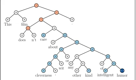
Figure 1: Example of the Recursive Neural Tensor Net-work accurately predicting 5 sentiment classes, very neg-ative to very positive (– –, –, 0, +, + +), at every node of a parse tree and capturing the negation and its scope in this sentence.

models to accurately capture the underlying phe-nomena presented in such data. To address this need, we introduce the Stanford Sentiment Treebank and a powerful Recursive Neural Tensor Network that can accurately predict the compositional semantic effects present in this new corpus.

The Stanford Sentiment Treebankis the first cor-pus with fully labeled parse trees that allows for a complete analysis of the compositional effects of sentiment in language. The corpus is based on the dataset introduced by Pang and Lee (2005) and consists of 11,855 single sentences extracted from movie reviews. It was parsed with the Stanford parser (Klein and Manning, 2003) and includes a total of 215,154 unique phrases from those parse trees, each annotated by 3 human judges. This new dataset allows us to analyze the intricacies of senti-ment and to capture complex linguistic phenomena. Fig. 1 shows one of the many examples with clear compositional structure. The granularity and size of

this dataset will enable the community to train com-positional models that are based on supervised and structured machine learning techniques. While there are several datasets with document and chunk labels available, there is a need to better capture sentiment from short comments, such as Twitter data, which provide less overall signal per document.

In order to capture the compositional effects with higher accuracy, we propose a new model called the Recursive Neural Tensor Network (RNTN). Recur-sive Neural Tensor Networks take as input phrases of any length. They represent a phrase through word vectors and a parse tree and then compute vectors for higher nodes in the tree using the same tensor-based composition function. We compare to several super-vised, compositional models such as standard recur-sive neural networks (RNN) (Socher et al., 2011b), matrix-vector RNNs (Socher et al., 2012), and base-lines such as neural networks that ignore word order, Naive Bayes (NB), bi-gram NB and SVM. All mod-els get a significant boost when trained with the new dataset but the RNTN obtains the highest perfor-mance with 80.7% accuracy when predicting fine-grained sentiment for all nodes. Lastly, we use a test set of positive and negative sentences and their re-spective negations to show that, unlike bag of words models, the RNTN accurately captures the sentiment change and scope of negation. RNTNs also learn that sentiment of phrases following the contrastive conjunction ‘but’ dominates.

The complete training and testing code, a live demo and the Stanford Sentiment Treebank dataset are available athttp://nlp.stanford.edu/

sentiment.

2 Related Work

This work is connected to five different areas of NLP research, each with their own large amount of related work to which we cannot do full justice given space constraints.

Semantic Vector Spaces. The dominant

ap-proach in semantic vector spaces uses distributional similarities of single words. Often, co-occurrence statistics of a word and its context are used to de-scribe each word (Turney and Pantel, 2010; Baroni and Lenci, 2010), such as tf-idf. Variants of this idea use more complex frequencies such as how often a

word appears in a certain syntactic context (Pado and Lapata, 2007; Erk and Pad´o, 2008). However, distributional vectors often do not properly capture the differences in antonyms since those often have similar contexts. One possibility to remedy this is to use neural word vectors (Bengio et al., 2003). These vectors can be trained in an unsupervised fashion to capture distributional similarities (Collobert and Weston, 2008; Huang et al., 2012) but then also be fine-tuned and trained to specific tasks such as sen-timent detection (Socher et al., 2011b). The models in this paper can use purely supervised word repre-sentations learned entirely on the new corpus.

Compositionality in Vector Spaces. Most of

the compositionality algorithms and related datasets capture two word compositions. Mitchell and La-pata (2010) use e.g. two-word phrases and analyze similarities computed by vector addition, multiplica-tion and others. Some related models such as holo-graphic reduced representations (Plate, 1995), quan-tum logic (Widdows, 2008), discrete-continuous models (Clark and Pulman, 2007) and the recent compositional matrix space model (Rudolph and Giesbrecht, 2010) have not been experimentally val-idated on larger corpora. Yessenalina and Cardie (2011) compute matrix representations for longer phrases and define composition as matrix multipli-cation, and also evaluate on sentiment. Grefen-stette and Sadrzadeh (2011) analyze subject-verb-object triplets and find a matrix-based categorical model to correlate well with human judgments. We compare to the recent line of work on supervised compositional models. In particular we will de-scribe and experimentally compare our new RNTN model to recursive neural networks (RNN) (Socher et al., 2011b) and matrix-vector RNNs (Socher et al., 2012) both of which have been applied to bag of words sentiment corpora.

Logical Form. A related field that tackles

com-positionality from a very different angle is that of trying to map sentences to logical form (Zettlemoyer and Collins, 2005). While these models are highly interesting and work well in closed domains and on discrete sets, they could only capture sentiment distributions using separate mechanisms beyond the currently used logical forms.

work on RNNs, several compositionality ideas re-lated to neural networks have been discussed by Bot-tou (2011) and Hinton (1990) and first models such as Recursive Auto-associative memories been exper-imented with by Pollack (1990). The idea to relate inputs through three way interactions, parameterized by a tensor have been proposed for relation classifi-cation (Sutskever et al., 2009; Jenatton et al., 2012), extending Restricted Boltzmann machines (Ranzato and Hinton, 2010) and as a special layer for speech recognition (Yu et al., 2012).

Sentiment Analysis. Apart from the

above-mentioned work, most approaches in sentiment anal-ysis use bag of words representations (Pang and Lee, 2008). Snyder and Barzilay (2007) analyzed larger reviews in more detail by analyzing the sentiment of multiple aspects of restaurants, such as food or atmosphere. Several works have explored sentiment compositionality through careful engineering of fea-tures or polarity shifting rules on syntactic strucfea-tures (Polanyi and Zaenen, 2006; Moilanen and Pulman, 2007; Rentoumi et al., 2010; Nakagawa et al., 2010).

3 Stanford Sentiment Treebank

Bag of words classifiers can work well in longer documents by relying on a few words with strong sentiment like ‘awesome’ or ‘exhilarating.’ How-ever, sentiment accuracies even for binary posi-tive/negative classification for single sentences has not exceeded 80% for several years. For the more difficult multiclass case including a neutral class, accuracy is often below 60% for short messages on Twitter (Wang et al., 2012). From a linguistic or cognitive standpoint, ignoring word order in the treatment of a semantic task is not plausible, and, as we will show, it cannot accurately classify hard ex-amples of negation. Correctly predicting these hard cases is necessary to further improve performance.

In this section we will introduce and provide some analyses for the newSentiment Treebankwhich in-cludes labels for every syntactically plausible phrase in thousands of sentences, allowing us to train and evaluate compositional models.

We consider the corpus of movie review excerpts from the rottentomatoes.com website orig-inally collected and published by Pang and Lee (2005). The original dataset includes 10,662

sen-nerdy  folks

| Very negative

|

Negative Somewhat| negative

|

Neutral Somewhat| positive

| Positive Very|

positive

phenomenal  fantasy  best  sellers

| Very negative

| Negative

| Somewhat

negative | Neutral

| Somewhat

positive | Positive

| Very positive  

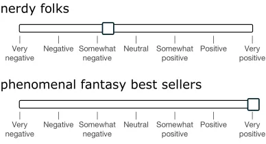
Figure 3: The labeling interface. Random phrases were shown and annotators had a slider for selecting the senti-ment and its degree.

tences, half of which were considered positive and the other half negative. Each label is extracted from a longer movie review and reflects the writer’s over-all intention for this review. The normalized, lower-cased text is first used to recover, from the origi-nal website, the text with capitalization. Remaining HTML tags and sentences that are not in English are deleted. The Stanford Parser (Klein and Man-ning, 2003) is used to parses all 10,662 sentences. In approximately 1,100 cases it splits the snippet into multiple sentences. We then used Amazon Me-chanical Turk to label the resulting 215,154 phrases. Fig. 3 shows the interface annotators saw. The slider has 25 different values and is initially set to neutral. The phrases in each hit are randomly sampled from the set of all phrases in order to prevent labels being influenced by what follows. For more details on the dataset collection, see supplementary material.

5 10 15 20 25 30 35 40 45 N-Gram Length

0% 20% 40% 60% 80% 100%

%

o

f S

en

tim

en

t V

al

ue

s

Neutral

Somewhat Positive

Positive

Very Positive

Somewhat Negative

Negative

Very Negative

(a)

(a) (b)

(b) (c)

(c) (d)

(d)

Distributions of sentiment values for (a) unigrams, (b) 10-grams, (c) 20-grams, and (d) full sentences.

Figure 2: Normalized histogram of sentiment annotations at eachn-gram length. Many shortern-grams are neutral; longer phrases are well distributed. Few annotators used slider positions between ticks or the extreme values. Hence the two strongest labels and intermediate tick positions are merged into 5 classes.

4 Recursive Neural Models

The models in this section compute compositional vector representations for phrases of variable length and syntactic type. These representations will then be used as features to classify each phrase. Fig. 4 displays this approach. When ann-gram is given to the compositional models, it is parsed into a binary tree and each leaf node, corresponding to a word, is represented as a vector. Recursive neural mod-els will then compute parent vectors in a bottom up fashion using different types of compositional-ity functions g. The parent vectors are again given as features to a classifier. For ease of exposition, we will use the tri-gram in this figure to explain all models.

We first describe the operations that the below re-cursive neural models have in common: word vector representations and classification. This is followed by descriptions of two previous RNN models and our RNTN.

Each word is represented as ad-dimensional vec-tor. We initialize all word vectors by randomly sampling each value from a uniform distribution:

U(−r, r), where r = 0.0001. All the word vec-tors are stacked in the word embedding matrixL∈

Rd×|V|, where|V|is the size of the vocabulary. Ini-tially the word vectors will be random but theL ma-trix is seen as a parameter that is trained jointly with the compositionality models.

We can use the word vectors immediately as parameters to optimize and as feature inputs to

a softmax classifier. For classification into five

classes, we compute the posterior probability over

not very good ...

a b c

p

=g(b,c)

p

= g(a,p

)

0 0 +

+ +

-Figure 4: Approach of Recursive Neural Network mod-els for sentiment: Compute parent vectors in a bottom up fashion using a compositionality functiongand use node vectors as features for a classifier at that node. This func-tion varies for the different models.

labels given the word vector via:

ya= softmax(Wsa), (1)

where Ws ∈ R5×d is the sentiment classification matrix. For the given tri-gram, this is repeated for vectors b and c. The main task of and difference between the models will be to compute the hidden vectorspi ∈Rdin a bottom up fashion.

4.1 RNN: Recursive Neural Network

The simplest member of this family of neural work models is the standard recursive neural net-work (Goller and K¨uchler, 1996; Socher et al., 2011a). First, it is determined which parent already has all its children computed. In the above tree ex-ample, p1 has its two children’s vectors since both

p1 =f

W

b c

, p2=f

W

a p1

,

wheref = tanhis a standard element-wise nonlin-earity, W ∈ _Rd×2d _{is the main parameter to learn}

and we omit the bias for simplicity. The bias can be added as an extra column toW if an additional1is added to the concatenation of the input vectors. The parent vectors must be of the same dimensionality to be recursively compatible and be used as input to the next composition. Each parent vectorpi, is given to

the samesoftmax classifier of Eq. 1 to compute its label probabilities.

This model uses the same compositionality func-tion as the recursive autoencoder (Socher et al., 2011b) and recursive auto-associate memories (Pol-lack, 1990). The only difference to the former model is that we fix the tree structures and ignore the re-construction loss. In initial experiments, we found that with the additional amount of training data, the reconstruction loss at each node is not necessary to obtain high performance.

4.2 MV-RNN: Matrix-Vector RNN

The MV-RNN is linguistically motivated in that most of the parameters are associated with words and each composition function that computes vec-tors for longer phrases depends on the actual words being combined. The main idea of the MV-RNN (Socher et al., 2012) is to represent every word and longer phrase in a parse tree as both a vector and a matrix. When two constituents are combined the matrix of one is multiplied with the vector of the other and vice versa. Hence, the compositional func-tion is parameterized by the words that participate in it.

Each word’s matrix is initialized as ad×didentity matrix, plus a small amount of Gaussian noise. Sim-ilar to the random word vectors, the parameters of these matrices will be trained to minimize the clas-sification error at each node. For this model, each n-gram is represented as a list of (vector,matrix) pairs, together with the parse tree. For the tree with (vec-tor,matrix) nodes:

(p2,P2)

(a,A) (p1,P1)

(b,B) (c,C)

the MV-RNN computes the first parent vector and its matrix via two equations:

p1 =f

W

Cb Bc

, P1 =f

WM

B C

,

whereWM ∈Rd×2dand the result is again ad×d matrix. Similarly, the second parent node is com-puted using the previously comcom-puted (vector,matrix) pair(p1, P1)as well as(a, A). The vectors are used

for classifying each phrase using the samesoftmax

classifier as in Eq. 1.

4.3 RNTN:Recursive Neural Tensor Network

One problem with the MV-RNN is that the number of parameters becomes very large and depends on the size of the vocabulary. It would be cognitively more plausible if there was a single powerful com-position function with a fixed number of parameters. The standard RNN is a good candidate for such a function. However, in the standard RNN, the input vectors only implicitly interact through the nonlin-earity (squashing) function. A more direct, possibly multiplicative, interaction would allow the model to have greater interactions between the input vectors.

Motivated by these ideas we ask the question: Can a single, more powerful composition function per-form better and compose aggregate meaning from smaller constituents more accurately than many in-put specific ones? In order to answer this question, we propose a new model called the Recursive Neu-ral Tensor Network (RNTN). The main idea is to use the same, tensor-based composition function for all nodes.

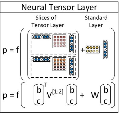
Fig. 5 shows a single tensor layer. We define the output of a tensor product h ∈ _Rd _{via the}

follow-ing vectorized notation and the equivalent but more detailed notation for each sliceV[i]_∈

Rd×d:

h=

b c

T

V[1:d]

b c

;hi =

b c

T

V[i]

b c

.

whereV[1:d] ∈ _R2d×2d×d _{is the tensor that defines}

Slices of Standard Tensor Layer Layer

p = f V

+ W

Neural Tensor Layer

b

c

b

c

b

c

T

p = f +

Figure 5: A single layer of the Recursive Neural Ten-sor Network. Each dashed box represents one ofd-many slices and can capture a type of influence a child can have on its parent.

The RNTN uses this definition for computingp1:

p1=f

b c

T

V[1:d]

b c

+W

b c

!

,

whereW is as defined in the previous models. The next parent vector p2 in the tri-gram will be

com-puted with the same weights:

p2 =f

a p1

T

V[1:d]

a p1

+W

a p1

!

.

The main advantage over the previous RNN model, which is a special case of the RNTN when V is set to0, is that the tensor can directly relate in-put vectors. Intuitively, we can interpret each slice of the tensor as capturing a specific type of compo-sition.

An alternative to RNTNs would be to make the compositional function more powerful by adding a second neural network layer. However, initial exper-iments showed that it is hard to optimize this model and vector interactions are still more implicit than in the RNTN.

4.4 Tensor Backprop through Structure

We describe in this section how to train the RNTN model. As mentioned above, each node has a

softmax classifier trained on its vector

representa-tion to predict a given ground truth or target vector t. We assume the target distribution vector at each node has a 0-1 encoding. If there areCclasses, then it has lengthCand a 1 at the correct label. All other entries are 0.

We want to maximize the probability of the cor-rect prediction, or minimize the cross-entropy error between the predicted distribution yi _∈

RC×1 at nodeiand the target distributionti ∈RC×1 at that node. This is equivalent (up to a constant) to mini-mizing the KL-divergence between the two distribu-tions. The error as a function of the RNTN parame-tersθ= (V, W, Ws, L)for a sentence is:

E(θ) =X

i

X

j

ti_jlogyi_j+λkθk2 ₍₂₎

The derivative for the weights of thesoftmax clas-sifier are standard and simply sum up from each node’s error. We definexi to be the vector at node i (in the example trigram, the xi ∈ _Rd×1_{’s are} (a, b, c, p1, p2)). We skip the standard derivative for

Ws. Each node backpropagates its error through to

the recursively used weightsV, W. Letδi,s ∈_Rd×1

be thesoftmaxerror vector at nodei:

δi,s= W_sT(yi−ti)

⊗f0(xi),

where⊗is the Hadamard product between the two vectors and f0 is the element-wise derivative of f which in the standard case of usingf = tanhcan be computed using onlyf(xi).

The remaining derivatives can only be computed in a top-down fashion from the top node through the tree and into the leaf nodes. The full derivative for V and W is the sum of the derivatives at each of the nodes. We define the complete incoming error messages for a node ias δi,com. The top node, in our casep2, only received errors from the top node’s

softmax. Hence, δp2,com _{= δ}p2,s _{which we can}

use to obtain the standard backprop derivative for W (Goller and K¨uchler, 1996; Socher et al., 2010). For the derivative of each slicek= 1, . . . , d, we get:

∂Ep2 ∂V[k] =δ

p2,com k

a p1

a p1

T

,

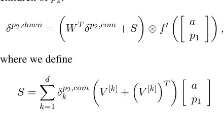
children ofp2:

δp2,down =

WTδp2,com+S

⊗f0

a p1

,

where we define

S =

d

X

k=1

δ_kp2,com

V[k]+

V[k]

T a

p1

The children ofp2, will then each take half of this

vector and add their ownsoftmaxerror message for the completeδ. In particular, we have

δp1,com =δp1,s+δp2,down[d+ 1 : 2d],

whereδp2,down[d+ 1 : 2d]indicates that p1 is the

right child ofp2and hence takes the 2nd half of the

error, for the final word vector derivative for a, it will beδp2,down[1 :d].

The full derivative for slice V[k]_{for this trigram}

tree then is the sum at each node:

∂E ∂V[k] =

Ep2 ∂V[k]+δ

p1,com k

b c

b c

T

,

and similarly forW. For this nonconvex optimiza-tion we use AdaGrad (Duchi et al., 2011) which con-verges in less than 3 hours to a local optimum.

5 Experiments

We include two types of analyses. The first type in-cludes several large quantitative evaluations on the test set. The second type focuses on two linguistic phenomena that are important in sentiment.

For all models, we use the dev set and cross-validate over regularization of the weights, word vector size as well as learning rate and minibatch size for AdaGrad. Optimal performance for all mod-els was achieved at word vector sizes between 25 and 35 dimensions and batch sizes between 20 and 30. Performance decreased at larger or smaller vec-tor and batch sizes. This indicates that the RNTN does not outperform the standard RNN due to sim-ply having more parameters. The MV-RNN has or-ders of magnitudes more parameters than any other model due to the word matrices. The RNTN would usually achieve its best performance on the dev set after training for 3 - 5 hours. Initial experiments

Model Fine-grained Positive/Negative All Root All Root

NB 67.2 41.0 82.6 81.8

SVM 64.3 40.7 84.6 79.4 BiNB 71.0 41.9 82.7 83.1 VecAvg 73.3 32.7 85.1 80.1 RNN 79.0 43.2 86.1 82.4 MV-RNN 78.7 44.4 86.8 82.9 RNTN 80.7 45.7 87.6 85.4

Table 1: Accuracy for fine grained (5-class) and binary predictions at the sentence level (root) and for all nodes.

showed that the recursive models worked signifi-cantly worse (over 5% drop in accuracy) when no nonlinearity was used. We usef = tanh in all ex-periments.

We compare to commonly used methods that use bag of words features with Naive Bayes and SVMs, as well as Naive Bayes with bag of bigram features. We abbreviate these with NB, SVM and biNB. We also compare to a model that averages neural word vectors and ignores word order (VecAvg).

The sentences in the treebank were split into a train (8544), dev (1101) and test splits (2210) and these splits are made available with the data release. We also analyze performance on only positive and negative sentences, ignoring the neutral class. This filters about 20% of the data with the three sets hav-ing 6920/872/1821 sentences.

5.1 Fine-grained Sentiment For All Phrases

The main novel experiment and evaluation metric analyze the accuracy of fine-grained sentiment clas-sification for all phrases. Fig. 2 showed that a fine grained classification into 5 classes is a reasonable approximation to capture most of the data variation. Fig. 6 shows the result on this new corpus. The RNTN gets the highest performance, followed by the MV-RNN and RNN. The recursive models work very well on shorter phrases, where negation and composition are important, while bag of features baselines perform well only with longer sentences. The RNTN accuracy upper bounds other models at mostn-gram lengths.

1*UDP/HQJWK

$F

FX

UD

F\

1*UDP/HQJWK

&X

P

XO

DW

LY

H

$F

FX

UD

F\

0RGHO 5171 09511 511 EL1% 1%

Figure 6: Accuracy curves for fine grained sentiment classification at eachn-gram lengths. Left: Accuracy separately for each set ofn-grams. Right: Cumulative accuracy of all≤n-grams.

5.2 Full Sentence Binary Sentiment

This setup is comparable to previous work on the original rotten tomatoes dataset which only used full sentence labels and binary classification of pos-itive/negative. Hence, these experiments show the improvement even baseline methods can achieve with the sentiment treebank. Table 1 shows results of this binary classification for both all phrases and for only full sentences. The previous state of the art was below 80% (Socher et al., 2012). With the coarse bag of words annotation for training, many of the more complex phenomena could not be captured, even by more powerful models. The combination of the new sentiment treebank and the RNTN pushes the state of the art on short phrases up to 85.4%.

5.3 Model Analysis: Contrastive Conjunction

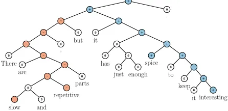
In this section, we use a subset of the test set which includes only sentences with an ‘X but Y’ structure: A phraseXbeing followed bybutwhich is followed by a phrase Y. The conjunction is interpreted as an argument for the second conjunct, with the first functioning concessively (Lakoff, 1971; Blakemore, 1989; Merin, 1999). Fig. 7 contains an example. We analyze a strict setting, whereXandY are phrases of different sentiment (including neutral). The ex-ample is counted as correct, if the classifications for both phrases X and Y are correct. Furthermore, the lowest node that dominates both of the word butand the node that spansY also have to have the same correct sentiment. For the resulting 131 cases, the RNTN obtains an accuracy of 41% compared to MV-RNN (37), RNN (36) and biNB (27).

5.4 Model Analysis: High Level Negation

We investigate two types of negation. For each type, we use a separate dataset for evaluation.

+ +

–

–

–

0

There

– 0

are

–

–

0

–

slow

0

and

–

repetitive

0

parts

0

,

0

but

+

0

it

+

0

0

has

0

0

just

0

enough

+

+

spice

+

0

to

+

0

keep

+

0

it

+

interesting

0

.

Figure 7: Example of correct prediction for contrastive conjunctionX but Y.

Set 1: Negating Positive Sentences. The first set

contains positive sentences and their negation. In this set, the negation changes the overall sentiment of a sentence from positive to negative. Hence, we compute accuracy in terms of correct sentiment re-versal from positive to negative. Fig. 9 shows two examples of positive negation the RNTN correctly classified, even if negation is less obvious in the case of ‘least’. Table 2 (left) gives the accuracies over 21 positive sentences and their negation for all models. The RNTN has the highest reversal accuracy, show-ing its ability to structurally learn negation of posi-tive sentences. But what if the model simply makes phrases very negative when negation is in the sen-tence? The next experiments show that the model captures more than such a simplistic negation rule.

Set 2: Negating Negative Sentences. The

ac-+ ac-+ 0 0 Roger 0 Dodger + + 0 is + 0 one + 0 of + + 0 the + + 0 most + compelling 0 variations 0 0 on 0 0 this 0 theme 0 . – 0 0 Roger 0 Dodger – – 0 is – 0 one – 0 of – – 0 the – – – least + compelling 0 variations 0 0 on 0 0 this 0 theme 0 . + 0 I + + + liked 0 0 0 every 0 0 single 0 minute 0 0 of 0 0 this 0 film 0 . – 0 I – – 0 0 did 0 n’t 0 0 like 0 0 0 a 0 0 single 0 minute 0 0 of 0 0 this 0 film 0 . – 0 It – – 0 0 ’s 0 just – + incredibly – – dull 0 . 0 0 It 0 0 0 0 0 ’s + definitely – not – – dull 0 .

Figure 9: RNTN prediction of positive and negative (bottom right) sentences and their negation.

Model Accuracy

Negated Positive Negated Negative

biNB 19.0 27.3

RNN 33.3 45.5

MV-RNN 52.4 54.6

RNTN 71.4 81.8

Table 2: Accuracy of negation detection. Negated posi-tive is measured as correct sentiment inversions. Negated negative is measured as increases in positive activations.

curacy in terms of how often each model was able to increase non-negative activation in the sentiment of the sentence. Table 2 (right) shows the accuracy. In over 81% of cases, the RNTN correctly increases the positive activations. Fig. 9 (bottom right) shows a typical case in which sentiment was made more positive by switching the main class from negative to neutral even though bothnotanddullwere nega-tive. Fig. 8 shows the changes in activation for both sets. Negative values indicate a decrease in

EL1% 551 09511 5171

1HJDWHG3RVLWLYH6HQWHQFHV&KDQJHLQ$FWLYDWLRQ

EL1% 551 09511 5171

1HJDWHG1HJDWLYH6HQWHQFHV&KDQJHLQ$FWLYDWLRQ

Figure 8: Change in activations for negations. Only the RNTN correctly captures both types. It decreases positive sentiment more when it is negated and learns that negat-ing negative phrases (such asnot terrible) should increase neutral and positive activations.

n Most positiven-grams Most negativen-grams

1 engaging; best; powerful; love; beautiful bad; dull; boring; fails; worst; stupid; painfully 2 excellent performances; A masterpiece; masterful

film; wonderful movie; marvelous performances

worst movie; very bad; shapeless mess; worst thing; instantly forgettable; complete failure 3 an amazing performance; wonderful all-ages

tri-umph; a wonderful movie; most visually stunning

for worst movie; A lousy movie; a complete fail-ure; most painfully marginal; very bad sign 5 nicely acted and beautifully shot; gorgeous

im-agery, effective performances; the best of the year; a terrific American sports movie; refresh-ingly honest and ultimately touching

silliest and most incoherent movie; completely crass and forgettable movie; just another bad movie. A cumbersome and cliche-ridden movie; a humorless, disjointed mess

8 one of the best films of the year; A love for films shines through each frame; created a masterful piece of artistry right here; A masterful film from a master filmmaker,

A trashy, exploitative, thoroughly unpleasant ex-perience ; this sloppy drama is an empty ves-sel.; quickly drags on becoming boring and pre-dictable.; be the worst special-effects creation of the year

Table 3: Examples ofn-grams for which the RNTN predicted the most positive and most negative responses.

1*UDP/HQJWK

$Y

HU

DJ

H

*

UR

XQ

G

7U

XW

K

6H

QW

LP

HQ

W 0RGHO

5171 09511 511

Figure 10: Average ground truth sentiment of top 10 most positiven-grams at variousn. The RNTN correctly picks the more negative and positive examples.

5.5 Model Analysis: Most Positive and

Negative Phrases

We queried the model for its predictions on what the most positive or negativen-grams are, measured as the highest activation of the most negative and most positive classes. Table 3 shows some phrases from the dev set which the RNTN selected for their strongest sentiment.

Due to lack of space we cannot compare top phrases of the other models but Fig. 10 shows that the RNTN selects more strongly positive phrases at mostn-gram lengths compared to other models.

For this and the previous experiment, please find additional examples and descriptions in the supple-mentary material.

6 Conclusion

We introduced Recursive Neural Tensor Networks and the Stanford Sentiment Treebank. The combi-nation of new model and data results in a system for single sentence sentiment detection that pushes state of the art by 5.4% for positive/negative sen-tence classification. Apart from this standard set-ting, the dataset also poses important new challenges and allows for new evaluation metrics. For instance, the RNTN obtains 80.7% accuracy on fine-grained sentiment prediction across all phrases and captures negation of different sentiments and scope more ac-curately than previous models.

Acknowledgments

References

M. Baroni and A. Lenci. 2010. Distributional mem-ory: A general framework for corpus-based semantics.

Computational Linguistics, 36(4):673–721.

Y. Bengio, R. Ducharme, P. Vincent, and C. Janvin. 2003. A neural probabilistic language model. J. Mach. Learn. Res., 3, March.

D. Blakemore. 1989. Denial and contrast: A relevance theoretic analysis of ‘but’. Linguistics and Philoso-phy, 12:15–37.

L. Bottou. 2011. From machine learning to machine reasoning. CoRR, abs/1102.1808.

S. Clark and S. Pulman. 2007. Combining symbolic and distributional models of meaning. InProceedings of the AAAI Spring Symposium on Quantum Interaction, pages 52–55.

R. Collobert and J. Weston. 2008. A unified architecture for natural language processing: deep neural networks with multitask learning. InICML.

J. Duchi, E. Hazan, and Y. Singer. 2011. Adaptive sub-gradient methods for online learning and stochastic op-timization. JMLR, 12, July.

K. Erk and S. Pad´o. 2008. A structured vector space model for word meaning in context. InEMNLP. C. Goller and A. K¨uchler. 1996. Learning

task-dependent distributed representations by backpropaga-tion through structure. InProceedings of the Interna-tional Conference on Neural Networks (ICNN-96). E. Grefenstette and M. Sadrzadeh. 2011. Experimental

support for a categorical compositional distributional model of meaning. InEMNLP.

E. Grefenstette, G. Dinu, Y.-Z. Zhang, M. Sadrzadeh, and M. Baroni. 2013. Multi-step regression learning for compositional distributional semantics. InIWCS. G. E. Hinton. 1990. Mapping part-whole hierarchies into

connectionist networks. Artificial Intelligence, 46(1-2).

L. R. Horn. 1989. A natural history of negation, volume 960. University of Chicago Press Chicago.

E. H. Huang, R. Socher, C. D. Manning, and A. Y. Ng. 2012. Improving Word Representations via Global Context and Multiple Word Prototypes. InACL. M. Israel. 2001. Minimizers, maximizers, and the

rhetoric of scalar reasoning. Journal of Semantics, 18(4):297–331.

R. Jenatton, N. Le Roux, A. Bordes, and G. Obozinski. 2012. A latent factor model for highly multi-relational data. InNIPS.

D. Klein and C. D. Manning. 2003. Accurate unlexical-ized parsing. InACL.

R. Lakoff. 1971. If’s, and’s, and but’s about conjunction. In Charles J. Fillmore and D. Terence Langendoen, ed-itors,Studies in Linguistic Semantics, pages 114–149. Holt, Rinehart, and Winston, New York.

A. Merin. 1999. Information, relevance, and social deci-sionmaking: Some principles and results of decision-theoretic semantics. In Lawrence S. Moss, Jonathan Ginzburg, and Maarten de Rijke, editors,Logic, Lan-guage, and Information, volume 2. CSLI, Stanford, CA.

J. Mitchell and M. Lapata. 2010. Composition in dis-tributional models of semantics. Cognitive Science, 34(8):1388–1429.

K. Moilanen and S. Pulman. 2007. Sentiment composi-tion. InIn Proceedings of Recent Advances in Natural Language Processing.

T. Nakagawa, K. Inui, and S. Kurohashi. 2010. Depen-dency tree-based sentiment classification using CRFs with hidden variables. InNAACL, HLT.

S. Pado and M. Lapata. 2007. Dependency-based con-struction of semantic space models. Computational Linguistics, 33(2):161–199.

B. Pang and L. Lee. 2005. Seeing stars: Exploiting class relationships for sentiment categorization with respect to rating scales. InACL, pages 115–124.

B. Pang and L. Lee. 2008. Opinion mining and senti-ment analysis. Foundations and Trends in Information Retrieval, 2(1-2):1–135.

T. A. Plate. 1995. Holographic reduced representations.

IEEE Transactions on Neural Networks, 6(3):623– 641.

L. Polanyi and A. Zaenen. 2006. Contextual valence shifters. In W. Bruce Croft, James Shanahan, Yan Qu, and Janyce Wiebe, editors,Computing Attitude and Af-fect in Text: Theory and Applications, volume 20 of

The Information Retrieval Series, chapter 1.

J. B. Pollack. 1990. Recursive distributed representa-tions.Artificial Intelligence, 46, November.

M. Ranzato and A. Krizhevsky G. E. Hinton. 2010. Factored 3-Way Restricted Boltzmann Machines For Modeling Natural Images. AISTATS.

V. Rentoumi, S. Petrakis, M. Klenner, G. A. Vouros, and V. Karkaletsis. 2010. United we stand: Improving sentiment analysis by joining machine learning and rule based methods. In Proceedings of the Seventh conference on International Language Resources and Evaluation (LREC’10), Valletta, Malta.

S. Rudolph and E. Giesbrecht. 2010. Compositional matrix-space models of language. InACL.

B. Snyder and R. Barzilay. 2007. Multiple aspect rank-ing usrank-ing the Good Grief algorithm. InHLT-NAACL. R. Socher, C. D. Manning, and A. Y. Ng. 2010. Learning

R. Socher, C. Lin, A. Y. Ng, and C.D. Manning. 2011a. Parsing Natural Scenes and Natural Language with Recursive Neural Networks. InICML.

R. Socher, J. Pennington, E. H. Huang, A. Y. Ng, and C. D. Manning. 2011b. Semi-Supervised Recursive Autoencoders for Predicting Sentiment Distributions. InEMNLP.

R. Socher, B. Huval, C. D. Manning, and A. Y. Ng. 2012. Semantic compositionality through recursive matrix-vector spaces. InEMNLP.

I. Sutskever, R. Salakhutdinov, and J. B. Tenenbaum. 2009. Modelling relational data using Bayesian clus-tered tensor factorization. InNIPS.

P. D. Turney and P. Pantel. 2010. From frequency to meaning: Vector space models of semantics. Journal of Artificial Intelligence Research, 37:141–188. H. Wang, D. Can, A. Kazemzadeh, F. Bar, and

S. Narayanan. 2012. A system for real-time twit-ter sentiment analysis of 2012 u.s. presidential elec-tion cycle. In Proceedings of the ACL 2012 System Demonstrations.

D. Widdows. 2008. Semantic vector products: Some ini-tial investigations. InProceedings of the Second AAAI Symposium on Quantum Interaction.

A. Yessenalina and C. Cardie. 2011. Composi-tional matrix-space models for sentiment analysis. In

EMNLP.

D. Yu, L. Deng, and F. Seide. 2012. Large vocabulary speech recognition using deep tensor neural networks. InINTERSPEECH.

F.M. Zanzotto, I. Korkontzelos, F. Fallucchi, and S. Man-andhar. 2010. Estimating linear models for composi-tional distribucomposi-tional semantics. InCOLING.