Abstract— This research proposes an efficient approach for solving the multiresponse problem in Taguchi method by aggressive formulation in data envelopment analysis. Each
experiment in Taguchi’s orthogonal array is treated as a decision making unit (DMU) with multiresponses set as inputs
and/or outputs. The efficiency of each DMU is then evaluated by aggressive formulation. Finally, the ordinal value of the DUM’s efficiency is used to decide the optimal combination of factor levels for multiresponse problem. Two case studies, which were investigated in previous literature, are provided for illustration. The computational results show that the proposed approach provides the largest anticipated improvement. In conclusion, the proposed approach may provide a great assistant to practitioners for solving the multiresponse problem in the manufacturing applications on Taguchi method.
Index Terms— Aggressive formulation, DEA, Multiresponse
problem, Taguchi method.
I. INTRODUCTION
Parameter design is a method, popularized by Taguchi [1], for designing products and manufacturing processes that are robust to uncontrollable variations. Taguchi method adopts a fractional factorial experimental design, called an orthogonal array (OA), which reduces the number of experiments under permissive reliability. Typically, the quality response of a process or a product can be divided into three main types: the smaller-the-better (STB); the nominal-the-best (NTB); and the larger-the-better (LTB) type response. Taguchi method has been found only efficient for optimizing a single response problem [2-3].
In today’s high competitive markets, most industries manufacture products with more than one quality response of main interest. Recently, optimizing multiresponse problem has received a considerable research attention. Therefore, several approaches [4-8] have been proposed to solve the multiresponse problem in Taguchi method. However, few approaches were reported efficient.
Data envelopment analysis (DEA) has been widely used for evaluating performance for a set of DMUs with multiple inputs and multiple outputs at organizational level, such as banks, hospitals, and universities [9]. DEA combines various
Manuscript received March 6, 2008. This work was supported by the Department of Industrial Engineering and Systems Management in Feng Chia University.
A. Al-Refaie is currently pursuing the Ph.D. degree in the Dept. of Industrial Engineering and Systems Management in Fen Chia University, Taiwan, R.O.C. (Corresponding author e-mail: eng_jo_2000@ yahoo.com). M.H. Li is a professor in the Dept. of Industrial Engineering and Systems Management in Fen Chia University, Taiwan, R.O.C.
inputs and various outputs for a DMU into one performance measure, called relative efficiency. Therefore, this research proposes an approach for solving the multiresponse problem in Taguchi method utilizing DEA techniques. DEA is introduced in the section II. The proposed approach is outlined in section III. Illustrations are provided in section IV. Finally, conclusions are summarized in section V.
II. DATA ENVELOPMENT ANALYSIS
DEA is a fractional mathematical programming technique for evaluating the relative efficiency of homogeneous DMUs with multiple inputs and multiple outputs. The most popular DEA technique is the CCR model, developed by Charnes, Cooper, and Rhodes [10]. The CCR model measures the relative efficiency of each DMU once by comparing it to a group of the other DMUs that have the same set of inputs and outputs. Assuming there are n DMUs each with m inputs and s outputs to be evaluated. Let the DMU to be individually evaluated on any trial be designated as DMUo. The relative
efficiency, Eoo, of DMUo with inputs of xio (i = 1, ... , m) and
outputs of yro (r = 1, ... , s) is evaluated by solving
1 1
1 1
1 2
Max = ( ) /( )
subject to ( ) /( ) 1 =1, ... , , , ... , 0
s m
oo r ro i io
r i
s m
r rj i ij
r i
s
E u y v x
u y v x j n
u u u
θ
= = = =
=
≤
≥
∑
∑
∑
∑
1 2
, , ... , v v vm≥0
where ur and vi are the virtual weights for the rth output and
ith input, respectively, and θ is a scalar. Obviously, the CCR model is nonlinear, which can be transformed into a linear model by setting the sum of the weighted inputs equal to one. The resulting model is called the “input-oriented” CCR model, which is expressed as
=1
=1
=1 =1
1 2
1 2
= Max =
subject to 1
=1, ... , , , ... , 0
, , ... , 0 s
oo r ro
r m
i io i
s m
r rj i ij
r i
s
m
E u y
v x
u y v x j n
u u u
v v v
θ
=
≤
≥ ≥
∑
∑
∑
∑
The objective function is the ratio of the sum of the weighted outputs. The first constraint ensures the sum of the weighted inputs is equal to one. Using the above model, DMUo is
identified as CCR-efficient if the relative efficiency Eoo
equals one. Baker and Talluri [11] showed that CCR model may provide misleading efficiency scores through identifying a DMU with an unrealistic weighing scheme to be efficient. Moreover, the Eoo may equal to one for more than
one DMU. As a result, the CCR-model fails to discriminate
Solving the Multiresponse Problem in Taguchi
Method by Aggressive Formulation in DEA
among efficient DMUs. In contrast, the aggressive formulation increases discrimination among efficient by allowing efficiency takes a value greater than one and allows for DMU’s peer-evaluation instead of self-evaluation [12]. A peer-evaluation means that DMUo is evaluated according to
the optimal weighting scheme of other DMUs. The main idea of aggressive formulation is to obtain a weighing scheme of DMUo that would be optimal in the CCR model, but have, as
a secondary objective, minimization of the cross-efficiencies of the other DMUs. The model of this technique given by
=1 = 1
= 1
1 1
1 1
Min ( . ) ( . )
subject to ( . ) 1
,
. =
s m
r o rj io ij
r j o i j o
m
io ij
i j o
s m
ro rj io ij
r i
s m
ro ro oo io io
r i
u y v x
v x
u y v x j o
u y E v x
δ
≠ ≠
≠ = =
= =
−
=
− ≤ ∀ ≠
−
∑ ∑
∑ ∑
∑ ∑
∑
∑
∑
∑
0 u vr o, io≥0where δ is a scalar, which is very close to zero. Utilizing the optimal uro and vio values, uro* andv*io, respectively, the cross-efficiencies of DMUo are then calculated. Let Eoj be the
cross-efficiency of DMUj calculated according to the optimal
weights of DMUo. The Eoj is calculated as
1 1
/
s m
oj ro rj io ij
r i
E u y v x
= =
=
∑
∑
j ≠ o (1)Let ej be the mean of cross-efficiencies for DMUj. The ej is
estimated as
/( 1) j oj
o j
e E n
≠
=
∑
− j = 1, ..., n (2)Once the Eoj and ej values are obtained, a matrix called the
“cross-efficiencies matrix” is constructed and used for comparing the performance of n DMUs. In this research, the aggressive formulation will be utilized for solving the multiresponse problem in Taguchi method.
III. PROPOSED APPROACH
The proposed approach for solving the multiresponse problem in Taguchi method is outlined in the following steps:
Step 1: Assume n experiments in Taguchi’s OA are conducted. Treat each experiment as a DMU. Typically, the efficiency is enhanced if the sum of the weighted outputs is increased and/or the sum of the weighted inputs is decreased. Therefore, set the multi-responses for each DMU based on the following:
i. If all responses are STB type, then set all responses as inputs, whereas set a unit (one) as the output. Conversely, if all responses are LTB type, then set all of them as the outputs, while set one as input.
ii. If all responses are NTB type, then calculate the estimate
where c is the quality loss coefficient, while yj and sj are
the average and standard deviation of response replicates for each DMUj, respectively. Set the Lj values as the
inputs and one as the output for all DMUs.
iii. If responses are a mix of the three types, set STB type response and Lj value of the NTB type response as
inputs, whereas set LTB type response(s) as the output.
Step 2: Obtain the Eoo value by solving the input-oriented
CCR model for each DMU.
Step 3: Estimate the *
ro
u and *
io
v values for each DMU by
solving aggressive formulation. Then, calculate the Eoj and ej
values using Eqs. (1) and (2), respectively. Finally, construct the cross-efficiencies matrix.
Step 4: Decide the ordinal value of ej. The ordinal value is to
rank the ej values such that the smallest ej value receives an
ordinal value of one, whereas the largest ej value takes an
ordinal value of n. Let AOVfl be the average of the ordinal
values at level l of factor f. Calculate the AOVfl value for
each factor level. Typically, higher AOVfl implies better
performance. Therefore, the optimal factor level is identified as the level that maximizes the value of AOVfl . If a tie occurs
in selecting the optimal level for a factor, then choose the factor level that provides the largest anticipated improvement as the optimal level for that factor.
Step 5: Calculate the anticipated improvement due to setting controllable factors at optimal levels obtained by aggressive formation.
IV. ILLUSTRATIONS
Two frequently-investigated case studies are provided to illustrate the proposed approach.
A- Optimization of Polysilicon Process
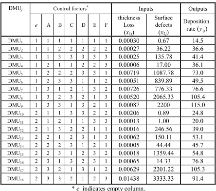
Taguchi method was used to improve the quality of polysilicon process [14] by optimizing concurrently three responses; the surface defects (STB), thickness (NTB, target is 3600 Å) and deposition rate (LTB). Six process factors were investigated simultaneously including: (A) deposition temperature, (B) deposition pressure, (C) Nitrogen flow, (D) silane flow, (E) settling time, and (F) cleaning method, utilizing L18 (21×37) array shown in Table 1. The proposed approach was adopted to optimize the three responses concurrently as follows:
Step 1: Each experiment in L18 (21×37) array is treated as a DMU. The quality loss of thickness, calculated using Eq. (3), and surface defects are set the inputs. Whereas, the deposition rate is set as the output for all DMUs.
Step 2: Each DMU is evaluated by solving the input-oriented CCR model. The Eoo (o = 1, ... , 18) is
displayed in Table 2. Note that all the Eoo values lie between
Step 3: Aggressive formulation model is adopted to evaluate the values of *
1j
v , *
2j,
v and *
1j
u for each DMUj. The results are
also shown in Table 2. For illustration, the values of
* 11
v , *
21,
v and *
11
u equal to 0.0, 0.00006892, and 0.00000318,
respectively, for DMU1 are obtained by solving
18 2 18
11 1
=2 = 1 =2
2 18
1
= 1 =2
2
11 1
1 2
11 1 11 1 1
1
Min ( ) ( . )
subject to ( . ) 1
, 2,...,18
= 0
rj i ij
j i j
i ij
i j
rj i ij
i
r i i
i
u y v x
v x
u y v x j
u y E v x
δ
= =
−
=
− ≤ =
−
∑
∑ ∑
∑ ∑
∑
∑
1 1
u vr, i ≥0
The values of * 1j
v , *
2j,
v and *
1j
u for other DMUs are obtained similarly. The Eoj and ej values are then calculated using
Eqs. (1) and (2) for each DMU. Finally, the cross-efficiencies matrix is constructed in Table 3. Note in Table 3, the DMUs identified as CCR-efficient have unequal ej values and hence
are no more equally efficient. This shows that the efficiency of the aggressive formulation technique in increasing the discrimination among efficient DMUs.
Step 4: The ordinal values for all ej values are decided and
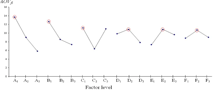
also listed in Table 3. The AOVfl valuesare then calculated
for all factor levels and plotted in Fig. 1. For illustration, the AOVA1, the efficiency of level 1 for factor A, is calculated as the average of the ordinal values for DMU1, DMU2, DMU3, DMU10, DMU11, and DMU12, then divided by six. From Fig. 1, it is clear that A1B1C1D2E2F2 is the combination of factor levels that optimizes the three responses concurrently. Table 1. Experimental data of polysilicon process.
Control factors* Inputs Outputs
DMUj
e A B C D E F
thickness Loss (x1j)
Surface defects
(x2j)
Deposition rate(y1j)
DMU1 1 1 1 1 1 1 1 0.00030 0.67 14.5
DMU2 1 1 2 2 2 2 2 0.00027 36.22 36.6
DMU3 1 1 3 3 3 3 3 0.00025 135.78 41.4
DMU4 1 2 1 1 2 2 3 0.00006 17.00 36.1
DMU5 1 2 2 2 3 3 1 0.00719 1087.78 73.0
DMU6 1 2 3 3 1 1 2 0.00051 839.89 49.5
DMU7 1 3 1 2 1 3 2 0.00726 776.33 76.6
DMU8 1 3 2 3 2 1 3 0.00520 2065.33 105.4
DMU9 1 3 3 1 3 2 1 0.00087 2200 115.0
DMU10 2 1 1 3 3 2 2 0.00206 0.89 24.8
DMU11 2 1 2 1 1 3 3 0.00013 1.00 20.0
DMU12 2 1 3 2 2 1 1 0.00016 246.56 39.0
DMU13 2 2 1 2 3 1 3 0.00062 150.11 53.1
DMU14 2 2 2 3 1 2 1 0.00005 44.44 45.7
DMU15 2 2 3 1 2 3 2 0.00018 1359.44 54.8
DMU16 2 3 1 3 2 3 1 0.00065 14.33 76.8
DMU17 2 3 2 1 3 1 2 0.00629 2201.22 105.3
DMU18 2 3 3 2 1 2 3 0.01438 3333.33 91.4
[image:3.612.316.538.56.252.2]* e indicates empty column.
Table 2. The results of aggressive formulation.
CCR-Model Aggressive Formulation
DMUj
Ejj δ v1*j
* 2j
v *
1j
u
DMU1 1.00000 0.000018 0.00000000 0.00006892 0.00000318
DMU2 0.38025 0.001007 0.00000000 0.00006909 0.00002600
DMU3 0.22037 0.000234 21.65440000 0.00000000 0.00002882
DMU4 1.00000 0.001507 0.00000000 0.00006900 0.00003249
DMU5 0.02626 0.001171 0.00000000 0.00007450 0.00002915
DMU6 0.09788 0.000000 21.77700000 0.00000000 0.00002196
DMU7 0.03359 0.000860 0.00000000 0.00007281 0.00002479
DMU8 0.03032 0.000445 24.25418000 0.00000000 0.00003628
DMU9 0.13343 0.000000 21.94908000 0.00000000 0.00002216
DMU10 1.00000 0.000000 0.00000000 0.00006892 0.00000247
DMU11 1.00000 0.000024 0.00000000 0.00006892 0.00000345
DMU12 0.25200 0.000000 21.61228000 0.00000000 0.00002234
DMU13 0.16001 0.001421 0.00000000 0.00006964 0.00003150
DMU14 1.00000 0.000000 21.56102000 0.00000000 0.00002359
DMU15 0.30722 0.000000 21.62162000 0.00000000 0.00002182
DMU16 0.67157 0.000153 0.00000000 0.00006898 0.00000864
DMU17 0.02609 0.000529 24.91281000 0.00000000 0.00003883
[image:3.612.73.540.502.692.2]DMU18 0.01227 0.001793 0.00000000 0.00008947 0.00004004
Table 3. The cross-efficiencies matrix by aggressive formulation for polysilicon process.
DMUj
DMUo DMU1 DMU2 DMU3 DMU4 DMU5 DMU6 DMU7 DMU8 DMU9 DMU10 DMU11 DMU12 DMU13 DMU14 DMU15 DMU16 DMU17 DMU18
DMU1 0.0467 0.0141 0.0981 0.003101 0.0027 0.0046 0.0024 0.0024 1.28756 0.9241 0.0073 0.0163 0.0475 0.0019 0.2476 0.0022 0.0013
DMU2 8.1438 0.1147 0.7991 0.025253 0.0222 0.0371 0.0192 0.0197 10.48572 7.5260 0.0595 0.1331 0.3870 0.0152 2.0167 0.0180 0.0103
DMU3 0.0643 0.1832 0.8049 0.013519 0.1288 0.0141 0.0270 0.1756 0.01598 0.2021 0.3317 0.1138 1.3162 0.4043 0.1567 0.0223 0.0085
DMU4 10.1914 0.4759 0.1436 0.031603 0.0278 0.0465 0.0240 0.0246 13.12210 9.4183 0.0745 0.1666 0.4843 0.0190 2.5238 0.0225 0.0129
DMU5 8.4685 0.3954 0.1193 0.8309 0.0231 0.0386 0.0200 0.0205 10.90372 7.8261 0.0619 0.1384 0.4024 0.0158 2.0971 0.0187 0.0107
DMU6 0.0487 0.1388 0.1670 0.6100 0.010245 0.0106 0.0204 0.1331 0.01211 0.1532 0.2513 0.0862 0.9974 0.3064 0.1188 0.0169 0.0064
DMU7 7.3675 0.3440 0.1038 0.7229 0.022846 0.0201 0.0174 0.0178 9.48613 6.8086 0.0538 0.1204 0.3501 0.0137 1.8245 0.0163 0.0093
DMU8 0.0722 0.2060 0.2477 0.9048 0.015196 0.1448 0.0158 0.1974 0.01797 0.2272 0.3728 0.1279 1.4795 0.4545 0.1762 0.0250 0.0095
DMU9 0.0487 0.1390 0.1672 0.6105 0.010255 0.0977 0.0107 0.0205 0.01212 0.1533 0.2516 0.0863 0.9984 0.3067 0.1189 0.0169 0.0064
DMU10 0.7767 0.0363 0.0109 0.0762 0.002408 0.0021 0.0035 0.0018 0.0019 0.7177 0.0057 0.0127 0.0369 0.0014 0.1923 0.0017 0.0010
DMU11 1.0821 0.0505 0.0152 0.1062 0.003355 0.0029 0.0049 0.0026 0.0026 1.39326 0.0079 0.0177 0.0514 0.0020 0.2680 0.0024 0.0014
DMU12 0.0499 0.1423 0.1712 0.6253 0.010503 0.1001 0.0109 0.0210 0.1364 0.01242 0.1570 0.0884 1.0225 0.3141 0.1218 0.0173 0.0066
DMU13 9.7894 0.4571 0.1379 0.9606 0.030356 0.0267 0.0446 0.0231 0.0236 12.60445 9.0467 0.0715 0.4652 0.0182 2.4242 0.0216 0.0124
DMU14 0.0528 0.1506 0.1812 0.6618 0.011115 0.1059 0.0116 0.0222 0.1444 0.01314 0.1662 0.2727 0.0936 0.3324 0.1289 0.0183 0.0070
DMU15 0.0487 0.1389 0.1671 0.6104 0.010251 0.0977 0.0107 0.0205 0.1332 0.01212 0.1533 0.2515 0.0863 0.9981 0.1188 0.0169 0.0064
DMU16 2.7119 0.1266 0.0382 0.2661 0.008409 0.0074 0.0124 0.0064 0.0066 3.49171 2.5061 0.0198 0.0443 0.1289 0.0051 0.0060 0.0034
DMU17 0.0753 0.2146 0.2581 0.9426 0.015832 0.1509 0.0165 0.0316 0.2057 0.01872 0.2367 0.3884 0.1333 1.5414 0.4735 0.1835 0.0099
DMU18 9.6843 0.4522 0.1364 0.9502 0.03003 0.0264 0.0442 0.0228 0.0234 12.46919 8.9497 0.0708 0.1583 0.4602 0.0180 2.3982 0.0214
ej 3.451546 0.217537 0.1290407 0.622386 0.014957 0.058069 0.01983 0.017806 0.0746 4.4328488 3.24542 0.15017 0.09551 0.65689 0.15897 0.88919 0.01556 0.0072595 Ordinal
Step 5: The anticipated improvement in each response due to setting factors at A1B1C1D2E2F2 and the anticipated improvements gained by other approaches in previous studies, including engineering judgment [14] the sum of the weighted normalized quality losses [13], PCA [5], and DEA based ranking (DEAR) [6], are displayed in Table 4. Clearly in Table 4, the largest anticipated
[image:4.612.129.481.182.332.2]improvements in thickness (= 14.84 dB) and surface defects (= 63.72 dB) correspond to the proposed approach. However, the largest anticipated improvement in deposition rate (= -9.34 dB) corresponds to the sum of the weighted of normalized quality losses. Nevertheless, among all techniques, the proposed approach provides the largest total anticipated improvement (= 69.22 dB). .
[image:4.612.81.530.383.476.2]Fig. 1. Optimal factor levels for polycilicon process (optimal level is identified by circle).
Table 4. The anticipated improvement for polysilicon process
Optimal condition (II) Anticipated improvement (II-I)
Quality response (dB) Starting condition
(I)
Engineering judgment
[ 14]
Sum of weighted quality loss
[13 ]
PCA
[ 5] DEAR [ 6] Proposed approach
Engineering judgment
[ 14]
Sum of weighted quality loss [13 ]
PCA
[ 5] DEAR [ 6] Proposed approach
Thickness 29.95 36.79 40.24 41.23 41.32 44.79 6.84 10.29 11.28 11.37 14.84
Surface defects -56.69 -19.84 -24.22 -2.29 1.20 7.03 36.85 32.47 54.40 57.89 63.72
Deposition rate 34.97 29.60 32.44 27.21 27.21 25.64 -5.37 -2.53 -7.76 -7.76 -9.34
Total anticipated improvement (dB) 38.32 40.23 57.92 61.5 69.22
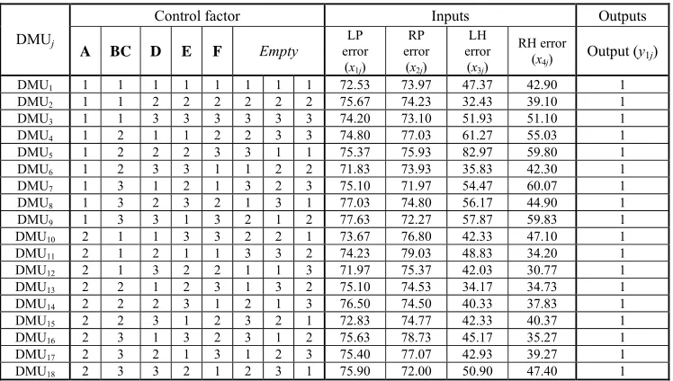
B- Optimization of Gear Hobbing Operation Genetic algorithm was employed to optimize four STB type responses of gear hobbing operation involving: left profile (LP) error, right profile (RP) error, left helix (LH) error, and right helix (RH) error [7]. Six controllable factors were investigated including: (A) direction of hobbing, (B) number of passes, (C) source of hob, (D) feed, (E) speed, and (F) job run out. The L18 (21×37) array was used for providing the layout of experimental work. Each experiment is treated as a DMU with LP error, RP error, LH error, and RH are set as the inputs, whereas a unit (one) is set as the output for all DMUs as shown in Table 5. The proposed approach to optimize the four responses concurrently is described briefly as follows. First, the Eoo values are
obtained by solving CCR model then displayed in Table 6. Then, the aggressive formulation is applied
to calculate the optimal input and output weights of each DMU. The Eoj values are computed for each
DMU. Then, the ej values with their corresponding
ordinal values are obtained and listed in the last two columns of Table 6. Finally, the AOVfl values are
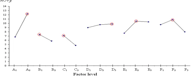
calculated and plotted in Fig. 2. In this figure, it is noted that A2B1C1D3E2F2 is the optimal combination of factor levels. Table 7 displays the anticipated improvement in each response at A2B1C1D3E2F2. The anticipated improvement gained by genetic approach [7] is also displayed in Table 7. The total anticipated improvement (= 11.2506 dB) due to setting factor levels at A2B1C1D3E2F2 larger than the anticipated improvement by genetic algorithm (= 4.1498 dB). Based on the above, it is concluded that the proposed approach is effective for solving the multiresponse problem in Taguchi method for gear hobbing operation.
Control factor Inputs Outputs DMUj
A BC D E F Empty
LP error
(x1j) RP error
(x2j) LH error
(x3j)
RH error
(x4j) Output (y1j)
DMU1 1 1 1 1 1 1 1 1 72.53 73.97 47.37 42.90 1
DMU2 1 1 2 2 2 2 2 2 75.67 74.23 32.43 39.10 1
DMU3 1 1 3 3 3 3 3 3 74.20 73.10 51.93 51.10 1
DMU4 1 2 1 1 2 2 3 3 74.80 77.03 61.27 55.03 1
DMU5 1 2 2 2 3 3 1 1 75.37 75.93 82.97 59.80 1
DMU6 1 2 3 3 1 1 2 2 71.83 73.93 35.83 42.30 1
DMU7 1 3 1 2 1 3 2 3 75.10 71.97 54.47 60.07 1
DMU8 1 3 2 3 2 1 3 1 77.03 74.80 56.17 44.90 1
DMU9 1 3 3 1 3 2 1 2 77.63 72.27 57.87 59.83 1
DMU10 2 1 1 3 3 2 2 1 73.67 76.80 42.33 47.10 1
DMU11 2 1 2 1 1 3 3 2 74.23 79.03 48.83 34.20 1
DMU12 2 1 3 2 2 1 1 3 71.97 75.37 42.03 30.77 1
DMU13 2 2 1 2 3 1 3 2 75.10 74.53 34.17 34.73 1
DMU14 2 2 2 3 1 2 1 3 76.50 74.50 40.33 37.83 1
DMU15 2 2 3 1 2 3 2 1 72.83 74.77 42.33 40.37 1
DMU16 2 3 1 3 2 3 1 2 75.63 78.73 45.17 35.27 1
DMU17 2 3 2 1 3 1 2 3 75.40 77.07 42.93 39.27 1
[image:5.612.120.494.66.278.2]DMU18 2 3 3 2 1 2 3 1 75.90 72.00 50.90 47.40 1
Table 6. The results of aggressive formulation.
Aggressive formulation (weights)
Inputs Output
DMUj CCR-Model(E
jj) *
1j
v *
2j
v *
3j
v *
4j
v *
1j
Fig. 2. Optimal factor levels for gear hobbing operation (optimal level is identified by circle).
Table 7. The anticipated improvement for gear hobbing operation.
Optimal condition (II) Anticipated improvement =(II) – (I) Quality
response (dB)
Initial condition
(I) Genetic algorithm
[7] Proposed approach
Genetic algorithm
[7] Proposed approach
LP error -37.8581 -37.4917 -37.1800 0.3664 0.6781
RP error -37.4952 -37.4045 -37.4984 0.0907 -0.0032
LH error -36.6009 -34.4082 -31.4320 2.1927 5.1688
RH error -35.7397 -34.2396 -30.3328 1.5001 5.4069
Total anticipated improvement (dB) 4.1498 11.2506
V. CONCLUSIONS
An effective approach for solving the multiresponse problem in Taguchi method is proposed in this research. Two case studies were presented for illustration. In conclusion, DEA techniques are not only efficient at organizational level, but also effective in manufacturing at operational level.
REFERENCES
[1] G. Taguchi, Taguchi Methods. Research and Development. Vol. 1. Dearborn, MI: American Suppliers Institute Press, 1991.
[2] C.C Tsao and H. Hocheng, “Comparison of the tool life of tungsten carbides coated by multi-layer TiCN and TiAlCN for end mills using the Taguchi method,” Journal of Material Processing Technology, vol. 123, 2002, pp. 1-4. [3] K.S. Anastasiou, “Optimization of the aluminium die
casting process based on the Taguchi method,” Proceedings of the Institution of Mechanical Engineers, vol. 216(7), 2002, pp. 969-977.
[4] C.T. Su and L.I. Tong, “Multi-response robust design by principal component analysis,” Total Quality Management, vol. 8(6), 1997, pp. 409–416.
[5] J. Antony, “Multi-response optimization in industrial experiments using Taguchi’s quality loss function and principal component analysis,” Quality and Reliability Engineering International, vol. 16, 2000, pp. 3–8. [6] H.C. Liao and Y.K. Chen, “Optimizing multi-response
problem in the Taguchi method by DEA based ranking method,” International Journal of Quality and Reliability
[7] R. Jeyapaul, P. Shahabudeen, and K. Krishnaiah, “Simultaneous optimization of multi-response problems in the Taguchi method using genetic algorithm,” International Journal of Advanced Manufacturing Technology, vol. 30, 2006, pp. 870–878.
[8] L.K. Pan, C.C. Wang, S.L. Wei, and H.F. Sher, “Optimizing multiple quality characteristics via Taguchi method-based grey analysis,” Journal of Materials Processing Technology, vol. 182, 2007, pp. 107–116.
[9] A. Charnes, W.W. Cooper, A.A. Letwin and L.M. Seiford,
Data Envelopment Analysis. Dordrecht: Kluwer, 1994. [10] A. Charnes, W.W. Cooper, and E. Rhodes, “Measuring the
efficiency of decision making units,” European Journal of Operational Research, vol. 2, 1978, pp. 429–444. [11] R.C. Baker and S. Talluri, “A closer look at the use of data
envelopment analysis for technology selection,” Computers and Industrial Engineering, vol. 28, 1997, pp. 101–108. [12] L. Angulo-Meza and M.P.E. Lins, “Review of Methods for
Increasing Discrimination in Data Envelopment Analysis,”
Annuals of Operations Research, vol. 116, 2002, pp.
225–242.
[13] L.I. Tong, C.T. Su, and C.H. Wang, “The optimization of multi-response problems in the Taguchi method,”
International Journal of Quality and Reliability Management, vol. 14(4), 1997, pp. 367–380.