Relevance Feedback Models for Recommendation
Masao Utiyama
National Institute of Information and Communications Technology 3-5 Hikari-dai, Soraku-gun, Kyoto 619-0289 Japan
Mikio Yamamoto
University of Tsukuba, 1-1-1 Tennodai, Tsukuba, 305-8573 Japan [email protected]
Abstract
We extended language modeling ap-proaches in information retrieval (IR) to combine collaborative filtering (CF) and content-based filtering (CBF). Our ap-proach is based on the analogy between IR and CF, especially between CF and rel-evance feedback (RF). Both CF and RF exploit users’ preference/relevance judg-ments to recommend items. We first in-troduce a multinomial model that com-bines CF and CBF in a language modeling framework. We then generalize the model to another multinomial model that approx-imates the Polya distribution. This gener-alized model outperforms the multinomial model by 3.4% for CBF and 17.4% for CF in recommending English Wikipedia articles. The performance of the gener-alized model for three different datasets was comparable to that of a state-of-the-art item-based CF method.
1 Introduction
Recommender systems (Resnick and Varian, 1997) help users select particular items (e.g, movies, books, music, and TV programs) that match their taste from a large number of choices by providing recommendations. The systems
ei-ther recommend a set of N items that will be of
interest to users (top-N recommendation problem) or predict the degree of users’ preference for items (prediction problem).
For those systems to work, they first have to aggregate users’ evaluations of items explicitly or implicitly. Users may explicitly evaluate certain movies as rating five stars to express their prefer-ence. These evaluations are used by the systems
asexplicit ratings (votes)of items or the systems infer the evaluations of items from the behavior of users and use these inferred evaluations asimplicit ratings. For example, systems can infer that users may like certain items if the systems learn which books they buy, which articles they read, or which TV programs they watch.
Collaborative filtering (CF) (Resnick et al.,
1994; Breese et al., 1998) andcontent-based (or
adaptive) filtering (CBF) (Allan, 1996; Schapire et al., 1998) are two of the most popular types of algorithms used in recommender systems. A CF system makes recommendations to current (active) users by exploiting their ratings in the
database. User-based CF (Resnick et al., 1994;
Herlocker et al., 1999) anditem-based CF(Sarwar et al., 2001; Karypis, 2001), among other CF algo-rithms, have been studied extensively. User-based CF first identifies a set of users (neighbors) that are similar to the active user in terms of their rat-ing patterns in the database. It then uses the neigh-bors’ rating patterns to produce recommendations for the active user. On the other hand, item-based CF calculates the similarity between items before-hand and then recommends items that are similar to those preferred by the active user. The perfor-mance of item-based CF has been shown to be comparable to or better than that of user-based CF (Sarwar et al., 2001; Karypis, 2001). In contrast to CF, CBF uses the contents (e.g., texts, genres, authors, images, and audio) of items to make rec-ommendations for the active user. Because CF and CBF are complementary, much work has been done to combine them (Basu et al., 1998; Yu et al., 2003; Si and Jin, 2004; Basilico and Hofmann, 2004).
The approach we took in this study is designed to solve top-N recommendation problems with
plicit ratings by using an item-based combination of CF and CBF. The methods described in this paper will be applied to recommending English Wikipedia1 articles based on those articles edited
by active users. (This is discussed in Section 3.) We use their editing histories and the contents of their articles to make top-N recommendations. We regard users’ editing histories as implicit ratings. That is, if users have edited articles, we consider that they have positive attitudes toward the arti-cles. Those implicit ratings are regarded as pos-itive examples. We do not have negative examples for learning their negative attitudes toward arti-cles. Consequently, handling our application with standard machine learning algorithms that require both positive and negative examples for classifica-tion (e.g., support vector machines) is awkward.
Our approach is based on the advancement in language modeling approaches to information re-trieval (IR) (Croft and Lafferty, 2003) and extends these to incorporate CF. The motivation behind our approach is the analogy between CF and IR, espe-cially between CF and relevance feedback (RF). Both CF and RF recommend items based on user preference/relevance judgments. Indeed, RF tech-niques have been applied to CBF, or adaptive fil-tering, successfully (Allan, 1996; Schapire et al., 1998). Thus, it is likely that RF can also be applied to CF.
To apply RF, we first extend the representation of items to combine CF and CBF under the models developed in Section 2. In Section 3, we report our experiments with the models. Future work and conclusion are in Sections 4 and 5.
2 Relevance feedback models
The analogy between IR and CF that will be ex-ploited in this paper is as follows.2 First, a
docu-ment in IR corresponds to an item in CF. Both are represented as vectors. A document is represented as a vector of words (bag-of-words) and an item is represented as a vector of user ratings (bag-of-user ratings). In RF, a (bag-of-user specifies documents that are relevant to his information need. These documents are used by the system to retrieve new
1http://en.wikipedia.org/wiki/Main Page 2The analogy between IR and CF has been recognized. For example, Breese et al. (1998) used the vector space model to measure the similarity between users in a user-based CF framework. Wang et al. (2005) used a language modeling approach different from ours. These works, however, treated only CF. In contrast with these, our model extends language modeling approaches to incorporate both CF and CBF.
relevant documents. In CF, an active user (implic-itly) specifies items that he likes. These items are used to search new items that will be preferred by the active user.
We userelevance models(Lavrenko and Croft,
2001; Lavrenko, 2004) as the basic framework of our relevance feedback models because (1) they perform relevance feedback well (Lavrenko, 2004) and (2) they can simultaneously handle dif-ferent kinds of features (e.g., difdif-ferent language texts (Lavrenko et al., 2002), such as texts and im-ages (Leon et al., 2003). These two points are es-sential in our application.
We first introduce a multinomial model follow-ing the work of Lavrenko (2004). This model is a novel one that extends relevance feedback ap-proaches to incorporate CF. It is like a combina-tion of relevance feedback (Lavrenko, 2004) and cross-language information retrieval (Lavrenko et al., 2002). We then generalize that model to an ap-proximated Polya distribution model that is better suited to CF and CBF. This generalized model is the main technical contribution of this work.
2.1 Preparation
Lavrenko (2004) adopts the method of kernels to
estimate probabilities: Let d be an item in the
database or training data, the probability of itemx
is estimated asp(x) = M1 Pdp(x|θd), whereM
is the number of items in the training data,θdis the
parameter vector estimated fromd, andp(x|θd)is the conditional probability of x givenθd.3 This
means that once we have defined a probability dis-tributionp(x|θ)and the method of estimatingθd
fromd, then we can assign probabilityp(x)tox
and apply language modeling approaches to CF and CBF.
To begin with, we define the representation
of item x as the concatenation of two vectors
{wx,ux}, where wx = wx1wx2. . . is the
se-quence of words (contents) contained in x and
ux = ux1ux2. . . is the sequence of users who have ratedximplicitly. We useVw andVu to
de-note the set of words and users in the database.
The parameter vector θis also the concatenation
of two vectors{ω, µ}, whereω andµare the pa-rameter vectors for Vw andVu, respectively. The probability of x given θ is defined as p(x|θ) = pω(wx|ω)pµ(ux|µ).
3Itemdin summationP
dand wordwin P
wand
Q
w
2.2 Multinomial model
Our first model regards that bothpωandpµfollow multinomial distributions. In this case,ω(w)and
µ(u) are the probabilities of wordw and user u. Then,pω(wx|ω)is defined as
pω(wx|ω) =
|wxY|
i=1
ω(wxi) = Y
w∈Vw
ω(w)n(w,wx)
(1) wheren(w,wx)is the number of occurrences ofw
inwx. In this model, we use a linear interpolation
method to estimate probabilityωd(w).
ωd(w) =λωPl(w|wd) + (1−λω)Pg(w) (2)
where Pl(w|wd) = Pn(w,wd)
w0n(w0,wd)
, Pg(w) = P
dn(w,wd) P
d P
w0n(w0,wd)
and λω (0 ≤ λω ≤ 1) is
a smoothing parameter. The estimation of user probabilities goes similarly: Letn(u,ux) be the
number of times user u implicitly rated item x,
we define or estimatepµ, λµ andµd in the same
way. In summary, we have defined a probability distribution p(x|θ) and the method of estimating
θd={ωd, µd}fromd.
To recommend top-N items, we have to rank items in the database in response to the implicit ratings of active users. We call those implicit rat-ingsqueryq. It is a set of items and is represented asq = {q1. . .qk}, where qi is an item
implic-itly rated by an active user andkis the size ofq. We next estimateθq ={ωq, µq}. Then, we com-pare θq andθd to rank items by using
Kullback-Leibler divergenceD(θq||θd)(Lafferty and Zhai,
2001; Lavrenko, 2004).
ωq(w)can be approximated as
ωq(w) = k1 k X
i=1
ωqi(w) (3)
where ωqi(w) is obtained by Eq. 2 (Lavrenko,
2004). However, we found in preliminary experi-ments that smoothing query probabilities hurt per-formance in our application. Thus, we use
ωqi(w) =Pl(w|wqi) =
n(w,wqi)
P
w0n(w0,wqi) (4)
instead of Eq. 2 whenqi is in a query.
Because KL-divergence is a distance measure, we use a score function derived from−D(θq||θd)
to rank items. We useSq(d) to denote the score
ofd givenq. Sq(d) is derived as follows. (We
ignore terms that are irrelevant to ranking items.)
−D(θq||θd) = −D(ωq||ωd)−D(µq||µd)
−D(ωq||ωd) rank= 1k k X
i=1
S(ωqi||ωd) (5)
where
S(ωqi||ωd) =
X
w
Pl(w|wqi)×log
µ
λωPl(w|wd)
(1−λω)Pg(w)+ 1
.
(6)
The summation goes over every word w that
is shared by both wqi and wd. We define
S(µqi||µd)similarly.4 Then, the score ofdgiven
qi,Sqi(d)is defined as
Sqi(d) =λsS(µqi||µd) + (1−λs)S(ωqi||ωd)
(7)
whereλs (0 ≤ λs ≤ 1)is a free parameter.
Fi-nally, the score ofdgivenqis
Sq(d) = 1k k X
i=1
Sqi(d). (8)
The calculation of Sq(d) can be very efficient
because once we cacheSqi(d) for each item pair ofqianddin the database, we can reuse it to
cal-culateSq(d)for any queryq. We further optimize
the calculation of top-N recommendations by stor-ing only the top 100 items (neighbors) in decreas-ing order of Sqi(·) for each item qi and setting the scores of lower ranked items as 0. (Note that
Sqi(d)>= 0holds.) Consequently, we only have to search small part of the search space without affecting the performance very much. These two types of optimization are common in item-based CF (Sarwar et al., 2001; Karypis, 2001).
2.3 Polya model
Our second model is based on the Polya
distribu-tion. We first introduce (hyper) parameter Θ =
{αω, αµ} and denote the probability of x given
Θ asp(x|Θ) = pω(wx|αω)pµ(ux|αµ). αω and
αµare the parameter vectors for words and users.
pω(wx|αω)is defined as follows.
pω(wx|αω) = Γ( P
wαωw)
Γ(Pwnx w+αωw)
Y
w
Γ(nxw+αwω) Γ(αω
w)
(9)
4S(µ
qi||µd) =
P
uPl(u|uqi) ×
log
³
λµPl(u|ud)
(1−λµ)Pg(u)+ 1
´
, where Pl(u|uqi) =
n(u,µqi)
P
u0n(u0,µqi)
, Pl(u|ud) = Pn(u,ud)
u0n(u0,ud), and
Pg(u) =
P
dn(u,ud)
P
d
P
u0n(u
0 1 2 3 4 5 6 7 8 9 10
0 2 4 6 8 100
1 2 3 4 5 6 7 8 9 10
nu(n,alpha)
n alpha=1e+5
alpha=38.8 alpha=16.4 alpha=9.0 alpha=5.4 alpha=3.3 alpha=2.0 alpha=1.1 alpha=0.4 alpha=1e-5
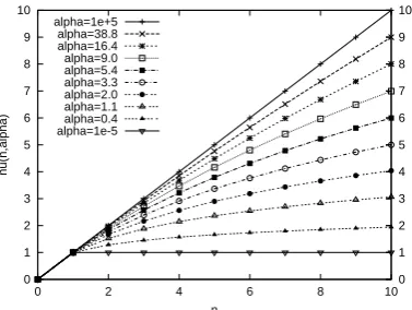
Figure 1: Relationship between original count n
and dumped countν(n, α)
whereΓis known as the gamma function,αω
wis a
parameter for wordwandnxw = n(w,wx). This
can be approximated as follows (Minka, 2003).
pω(wx|αω)∼ Y
w
ω(w)n˜(w,wx) (10)
where
˜
n(w,wx) = αωw(Ψ(nxw+αωw)−Ψ(αωw))
≡ ν(nxw, αωw) (11)
Ψis known as the digamma function and is
sim-ilar to the natural logarithm. We call Eq. 10 the approximated Polya model or simply the Polya model in this paper.
Eq. 10 indicates that the Polya distribution can be interpreted as a multinomial distribution over a modified set of counts˜n(·)(Minka, 2003).
[image:4.595.86.275.58.200.2]These modified counts are dumped as shown in
Fig. 1. Whenαωw → ∞, ν(nxw, αωw) approaches
nx
w. When αωw → 0, ν(nwx, αωw) = 0 if nxw = 0
otherwise it is 1. For intermediate values of αω w,
the mappingνdumps the original counts.
Under the approximation of Eq. 10, the es-timation of parameters can be understood as the maximum-likelihood estimate of a multinomial
distribution from dumped counts n(˜ ·) (Minka,
2003). Indeed, all we have to do to estimate the parameters for ranking items is replacePl andPg
from Section 2.2 withPl(w|wd) = Pn˜(w,wd)
w0n˜(w0,wd)
,
Pg(w) = P
d˜n(w,wd) P
d P
w0n˜(w0,wd)
, and Pl(w|wqi) = ˜
n(w,wqi)
P
w0n˜(w0,wqi)
. Then, as in the multinomial model, we can defineS(ωqi||ωd)with these probabilities. This argument also applies toS(µqi||µd).
The approximated Polya model is a generaliza-tion of the multinomial model described in Sec-tion 2.2. If we setαωw andαµu very large then the Polya model is identical to the multinomial model. By comparing Eqs. 1 and 10, we can see why the Polya model is superior to the multinomial model for modeling the occurrences of words (and users). In the multinomial model, if a word with probabil-itypoccurs twice, its probability becomesp2. In the Polya model, the word’s probability becomes
p1.5, for example, if we set αω
w = 1. Clearly,
p2 < p1.5; therefore, the Polya model assigns higher probability. In this example, the Polya model assigns probabilitypto the first occurrence andp0.5(> p)to the second. Since words that oc-cur once are likely to ococ-cur again (Church, 2000), the Polya model is better suited to model the oc-currences of words and users. See Yamamoto and Sadamitsu (2005) for further discussion on apply-ing the Polya distribution to text modelapply-ing.
Zaragoza et al.(2003) applied the Polya distri-bution to ad hoc IR. They introduced the exact Polya distribution (see Eq. 9) as an extension to the Dirichlet prior method (Zhai and Lafferty, 2001). However, we have introduced a multino-mial approximation of the Polya distribution. This approximation allows us to use the linear interpo-lation method to mix the approximated Polya dis-tributions. Thus, our model is similar to two-stage language models (Zhai and Lafferty, 2002) that combine the Dirichlet prior method and the lin-ear interpolation method. In contrast to our model, Zaragoza et al.(2003) had difficulty in mixing the Polya distributions and did not treat that in their paper.
3 Experiments
We first examined the behavior of the Polya model by varying the parameters. We tiedαωw for every
wandαµ
u for everyu; for anywandu,αωw =αω
andαµ
u =αµ. We then compared the Polya model
to an item-based CF method.
3.1 Behavior of Polya model 3.1.1 Dataset
We made a dataset of articles from English
Wikipedia5 to evaluate the Polya model. English
Wikipedia is an online encyclopedia that anyone
5We downloaded 20050713 pages full.xml.gz and 20050713 pages current.xml.gz from
can edit, and it has many registered users. Our aim is to recommend a set of articles to each user that is likely to be of interest to that user. If we can successfully recommend interesting articles, this could be very useful to a wide audience cause Wikipedia is very popular. In addition, be-cause wikis are popular media for sharing knowl-edge, developing effective recommender systems for wikis is important.
In our Wikipedia dataset, each item (article)x
consisted ofwxandux. uxwas the sequence of
users who had editedx. If users had editedx mul-tiple times, then those users occurred inux multi-ple times.wxwas the sequence of words that were
typical inx. To makewx, we removed stop words
and stemmed the remaining words with a Porter stemmer. Next, we identified 100 typical words in each article and extracted only those words
(|wx| ≥ 100 because some of them occurred
multiple times). Typicality was measured using the log-likelihood ratio test (Dunning, 1993). We needed to reduce the number of words to speed up our recommender system.
To make our dataset, we first extracted 302,606 articles, which had more than 100 tokens after the stop words were removed. We then selected typi-cal words in each article. The implicit rating data were obtained from the histories of users editing these articles. Each rating consisted of{user, ar-ticle, number of edits}. The size of this original rating data was 3,325,746. From this data, we ex-tracted a dense subset that consisted of users and articles included in at least 25 units of the original data. We discarded the users who had edited more than 999 articles because they were often software robots or system operators, not casual users. The resulting 430,096 ratings consisted of 4,193 users and 9,726 articles. Each user rated (edited) 103 articles on average (the median was 57). The av-erage number of ratings per item was 44 and the median was 36.
3.1.2 Evaluation of Polya model
We conducted a four-fold cross validation of this rating dataset to evaluate the Polya model. We used three-fourth of the dataset to train the model and one-fourth to test it.6 All users who existed in
6We needed to estimate probabilities of users and words. We used only training data to estimate the probabilities of users. However, we used all 9,726 articles to estimate the probabilities of words because the articles are usually avail-able even when editing histories of users are not.
both training and test data were used for evalua-tion. For each user, we regarded the articles in the training data that had been edited by the user as a query and ranked articles in response to it. These ranked top-N articles were then compared to the articles in the test data that were edited by the same user to measure the precisions for the user.
We used P@N (precision at rankN = the ratio of
the articles edited by the user in the top-N articles), S@N (success at rankN= 1 if some top-N articles were edited by the user, else 0), and R-precision (=
P@N, whereN is the number of articles edited by
the user in the test data). These measures for each user were averaged over all users to get the mean precision of each measure. Then, these mean pcisions were averaged over the cross validation re-peats.
Here, we report the averaged mean
pre-cisions with standard deviations. We first
report how R-precision varied
depend-ing on α (αω or αµ). α was varied over
10−5,0.4,1.1,2,3.3,5.4,9,16.4,38.8, and 105.
The values of ν(10, α) were approximately 1, 2,
3, 4, 5, 6, 7, 8, 9, and 10, respectively, as shown
in Fig. 1. When α = 105, the Polya model
represents the multinomial model as discussed in Section 2.3. For each value ofα, we variedλ(λω
orλµ) over 0.01, 0.05, 0.1, 0.2, 0.3, 0.4, 0.5, 0.6,
0.7, 0.8, 0.9, 0.95, and 0.99 to obtain the optimum
R-precision. These optimum R-precisions are
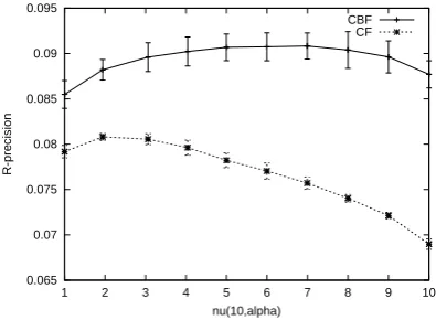
shown in Fig. 2. In this figure, CBF and CF represent the R-precisions for the content-based and collaborative filtering part of the Polya model. The values of CBF and CF were obtained by
setting λs = 0 and λs = 1 in Eq. 7 (which
is applied to the Polya model instead of the multinomial model), respectively. The error bars represent standard deviations.
At once, we noticed that CBF outperformed CF. This is reasonable because the contents of Wikipedia articles should strongly reflect the users (authors) interest. In addition, each article had about 100 typical words, and this was richer than the average number of users per article (44). This observation contrasts with other work where CBF performed poorly compared with CF, e.g., (Ali and van Stam, 2004).
Another important observation is that both
curves in Fig. 2 are concave. The best
R-precisions were obtained at intermediate values of
0.065 0.07 0.075 0.08 0.085 0.09 0.095
1 2 3 4 5 6 7 8 9 10
R-precision
nu(10,alpha)
[image:6.595.320.517.58.204.2]CBF CF
Figure 2: R-precision for Polya model
Table 1: Improvement in R-precision (RP) best RP (ν(·)/α) RP (ν(·)/α) %change CBF 0.091 (7/9.0) 0.088 (10/105) +3.4%
CF 0.081 (2/0.4) 0.069 (10/105) +17.4%
When α = 105 orν(10, α) ∼ 10, the Polya model represents the multinomial model as dis-cussed in Section 2.3. Thus, Fig. 2 and Table 1 show that the best R-precisions achieved by the Polya model were better than those obtained by the multinomial model. The improvement was 3.4% for CBF and 17.4% for CF as shown in Ta-ble 1. The improvement of CF was larger than that of CBF. This implies that the occurrences of users are more clustered than those of words. In other words, the degree of repetition in the editing histories of users is greater than that in word se-quences. A user who edits an article are likely to edit the article again.
From Fig. 2 and Table 1, we concluded that the generalization of a multinomial model achieved by the Polya model is effective in improving recom-mendation performance.
3.1.3 Combination of CBF and CF
Next, we show how the combination of CBF and CF improves recommendation performance. We set α (αω andαµ) to the optimum values in
Table 1 and variedλ(λs,λωandλµ) to obtain the R-precisions for CBF+CF, CBF and CF in Fig. 3. The values of CBF were obtained as follows. We first setλs = 0 in Eq. 7 to use only CBF scores
and then varied λω, which is the smoothing
pa-rameter for word probabilities, in Eq. 2. To get the values of CF, we setλs = 1in Eq. 7 and then varied λµ, which is the smoothing parameter for
user probabilities. The values of CBF+CF were obtained by varyingλsin Eq. 7 while settingλω
andλµto the optimum values obtained from CBF
0.055 0.06 0.065 0.07 0.075 0.08 0.085 0.09 0.095 0.1
0 0.1 0.2 0.3 0.4 0.5 0.6 0.7 0.8 0.9 1
R-precision
lambda
CBF+CF CBF CF
[image:6.595.84.282.59.204.2]Figure 3: Combination of CBF and CF.
Table 2: Precision and Success at top-N
CBF+CF CBF CF
N P@N S@N P@N S@N P@N S@N
5 0.166 0.470 0.149 0.444 0.137 0.408
10 0.135 0.585 0.123 0.562 0.112 0.516
15 0.117 0.650 0.107 0.628 0.098 0.582
20 0.105 0.694 0.096 0.671 0.089 0.627
R-precision 0.099 0.091 0.081
optimumλ λs= 0.2 λω= 0.01 λµ= 0.2
and CF (see Table 2). These parameters (λs, λω
andλµ) were defined in the context of the
multi-nomial model in Section 2.2 and used similarly in the Polya model in this experiment.
We can see that the combination was quite ef-fective as CBF+CF outperformed both CBF and CF. Table 2 shows R-precision, P@N and S@N forN = 5,10,15,20. These values were obtained by using the optimum values ofλin Fig. 3.
Table 2 shows the same tendency as Fig. 3. For
all values ofN, CBF+CF outperformed both CBF
and CF. We attribute this effectiveness of the com-bination to the feature independence of CBF and CF. CBF used words as features and CF used user ratings as features. They are very different kinds of features and thus can provide complementary information. Consequently, CBF+CF can exploit the benefits of both methods. We need to do fur-ther work to confirm this conjecture.
3.2 Comparison with a baseline method
We compared the Polya model to an implementa-tion of a state-of-the-art item-based CF method,
CProb (Karypis, 2001). CProb has been tested with various datasets and found to be effective in top-N recommendation problems. CProb has also been used in recent work as a baseline method (Ziegler et al., 2005; Wang et al., 2005).
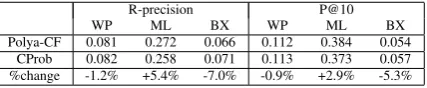
[image:6.595.312.521.251.332.2]R-precision P@10
WP ML BX WP ML BX
Polya-CF 0.081 0.272 0.066 0.112 0.384 0.054
CProb 0.082 0.258 0.071 0.113 0.373 0.057
[image:7.595.76.290.62.106.2]%change -1.2% +5.4% -7.0% -0.9% +2.9% -5.3%
Table 3: Comparison of Polya-CF and CProb
the 1 million MovieLens dataset.7 This data
con-sists of 1,000,209 ratings of 3,706 movies by 6,040 users. Each user rated an average of 166 movies (the median was 96). The average number of rat-ings per movie was 270 and the median was 124. The second was the BookCrossing dataset (Ziegler et al., 2005). This data consists of 1,149,780 rat-ings of 340,532 books by 105,283 users. From this data, we removed books rated by less than 20 users. We also removed users who rated less than 5 books. The resulting 296,471 ratings consisted of 10,345 users and 5,943 books. Each user rated 29 books on average (the median was 10). The av-erage number of ratings per book was 50 and the median was 33. Note that in our experiments, we regarded the ratings of these two datasets as im-plicit ratings. We regarded the number of occur-rence of each rating as one.
We conducted a four-fold cross validation for each dataset to compare CProb and Polya-CF, which is the collaborative filtering part of the Polya model as described in the previous section. For each cross validation repeat, we tuned the pa-rameters of CProb and Polya-CF on the test data to get the optimum R-precisions, in order to compare
best results for these models.8 P@N and S@N
were calculated with the same parameters. These measures were averaged as described above. R-precision and P@10 are in Table 3. The max-imum standard deviation of these measures was 0.001. We omitted reporting other measures be-cause they had similar tendencies. In Table 3, WP, ML and BX represent the Wikipedia, MovieLens, and BookCrossing datasets.
In Table 3, we can see that the variation of per-formance among datasets was greater than that be-tween Polya-CF and CProb. Both methods
per-7http://www.grouplens.org/
8CProb has two free parameters. Polya-CF also has two free parameters (αµandλµ). However, for MovieLens and
BookCrossing datasets, Polya-CF has only one free parame-terλµ, because we regarded the number of occurrence of each
rating as one, which meansν(1, αµ) = 1for allαµ>0(See
Fig. 1). Consequently, we don’t have to tuneαµ. Since the
number of free parameters is small, the comparison of perfor-mance shown in Table 3 is likely to be reproduced when we tune the parameters on separate development data instead of test data.
formed best against ML. We think that this is be-cause ML had the densest ratings. The average number of ratings per item was 270 for ML while that for WP was 44 and that for BX was 50.
Table 3 also shows that Polya-CF outperformed CProb when the dataset was ML and CProb was better than Polya-CF in the other cases. However, the differences in precision were small. Overall, we can say that the performance of Polya-CF is comparable to that of CProb.
An important advantage of the Polya model over CProb is that the Polya model can unify CBF and CF in a single language modeling framework while CProb handles only CF. Another advantage of the Polya model is that we can expect to im-prove its performance by incorporating techniques developed in IR because the Polya model is based on language modeling approaches in IR.
4 Future work
We want to investigate two areas in our future work. One is the parameter estimation and the other is the refinement of the query model.
We tuned the parameters of the Polya model by exhaustively searching the parameter space guided
by R-precision. We actually tried to learn αω
and αµ from the training data by using an EM
method (Minka, 2003; Yamamoto and Sadamitsu, 2005). However, the estimated parameters were about 0.05, too small for better recommendations. We need further study to understand the relation between the probabilistic quality (perplexity) of the Polya model and its recommendation quality.
We approximate the query model as Eq. 3. This allows us to optimize score calculation consider-ably. However, this does not consider the interac-tion among items, which may deteriorate the qual-ity of probabilqual-ity estimation. We want to inves-tigate more efficient query models in our future work.
5 Conclusion
gen-eralization of the multinomial model and showed that it is better suited to CF and CBF. The perfor-mance of the Polya model is comparable to that of a state-of-the-art item-based CF method.
Our work shows that language modeling ap-proaches in information retrieval can be extended to CF. This implies that a large amount of work in the field of IR could be imported into CF. This would be interesting to investigate in future work.
References
Kamal Ali and Wijnand van Stam. 2004. TiVo: Mak-ing show recommendations usMak-ing a distributed col-laborative filtering architecture. InKDD’04.
James Allan. 1996. Incremental relevance feedback for information filtering. InSIGIR’96.
Justin Basilico and Thomas Hofmann. 2004. Uni-fying collaborative and content-based filtering. In
ICML’04.
Chumki Basu, Haym Hirsh, and William Cohen. 1998. Recommendation as classification: Using social and content-based information in recommendation. In
AAAI-98.
John S. Breese, David Heckerman, and Carl Kadie. 1998. Empirical analysis of predictive algorithms for collaborative filtering. Technical report, MSR-TR-98-12.
Kenneth W. Church. 2000. Empirical estimates of adaptation: The chance of two Noriegas is closer to
p/2thanp2. InCOLING-2000, pages 180–186.
W. Bruce Croft and John Lafferty, editors. 2003. Lan-guage Modeling for Information Retrieval. Kluwer Academic Publishers.
Ted Dunning. 1993. Accurate methods for the
statis-tics of surprise and coincidence. Computational
Linguistics, 19(1):61–74.
Jonathan L. Herlocker, Joseph A. Konstan,
Al Borchers, and John Riedl. 1999. An
algo-rithmic framework for performing collaborative filtering. InSIGIR’99, pages 230–237.
George Karypis. 2001. Evaluation of item-based
top-N recommendation algorithms. InCIKM’01.
John Lafferty and ChengXiang Zhai. 2001. Document language models, query models and risk minimiza-tion for informaminimiza-tion retrieval. InSIGIR’01.
Victor Lavrenko and W. Bruce Croft. 2001.
Relevance-based language models. InSIGIR’01.
Victor Lavrenko, Martin Choquette, and W. Bruce Croft. 2002. Cross-lingual relevance models. In
SIGIR’02, pages 175–182.
Victor Lavrenko. 2004. A Generative Theory of
Rele-vance. Ph.D. thesis, University of Massachusetts.
J. Leon, V. Lavrenko, and R. Manmatha. 2003. Au-tomatic image annotation and retrieval using
cross-media relevance models. InSIGIR’03.
Thomas P. Minka. 2003.
Es-timating a Dirichlet distribution.
http://research.microsoft.com/˜minka/papers/dirichlet/.
Paul Resnick and Hal R. Varian. 1997. Recommender
systems. Communications of the ACM, 40(3):56–
58.
Paul Resnick, Neophytos Iacovou, Mitesh Suchak, Pe-ter Bergstrom, and John Riedl. 1994. GroupLens: An open architecture for collaborative filtering of
netnews. InCSCW’94, pages 175–186.
Badrul Sarwar, George Karypis, Joseph Konstan, and John Riedl. 2001. Item-based collaborative filtering
recommendation algorithms. InWWW10.
Robert E. Schapire, Yoram Singer, and Amit Singhal. 1998. Boosting and Rocchio applied to text filtering. InSIGIR’98, pages 215–223.
Luo Si and Rong Jin. 2004. Unified filtering by com-bining collaborative filtering and content-based fil-tering via mixture model and exponential model. In
CIKM-04, pages 156–157.
Jun Wang, Marcel J.T. Reinders, Reginald L.
La-gendijk, and Johan Pouwelse. 2005.
Self-organizing distributed collaborative filtering. In SI-GIR’05, pages 659–660.
Mikio Yamamoto and Kugatsu Sadamitsu. 2005.
Dirichlet mixtures in text modeling. Technical re-port, University of Tsukuba, CS-TR-05-1.
Kai Yu, Anton Schwaighofer, Volker Tresp, Wei-Ying Ma, and HongJiang Zhang. 2003. Collaborative ensemble learning: Combining collaborative and content-based information filtering via hierarchical
Bayes. InUAI-2003.
Hugo Zaragoza, Djoerd Hiemstra, and Michael Tip-ping. 2003. Bayesian extension to the language model for ad hoc information retrieval. InSIGIR’03.
ChengXiang Zhai and John Lafferty. 2001. A study of smoothing methods for language models applied to ad hoc information retrieval. InSIGIR’01.
ChengXiang Zhai and John Lafferty. 2002. Two-stage
language models for information retrieval. In
SI-GIR’02, pages 49–56.
Cai-Nicolas Ziegler, Sean M. McNee, Joseph A. Kon-stan, and Georg Lausen. 2005. Improving rec-ommendation lists through topic diversification. In